Quantum CFD at QCE26 learned the price of its doors

This guide follows 23 talks on quantum computing for fluid dynamics and other differential equations at IEEE Quantum Week 2026 in Toronto. The sharpest numbers priced getting data in and out, and the solve between.

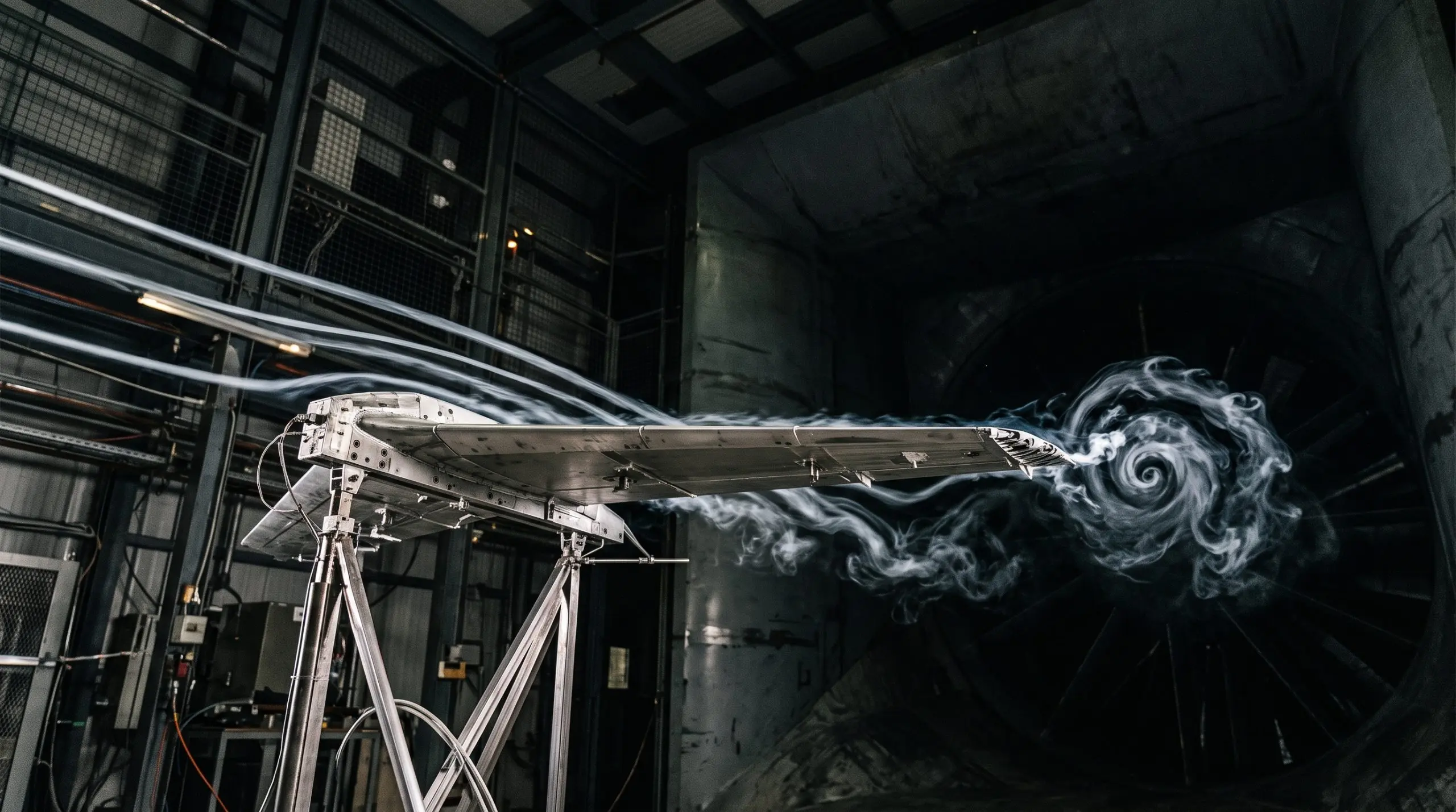
On Sunday 13 September, in Room 701B, Krishnan Suresh of the University of Wisconsin-Madison gave the first talk of a day on quantum CFD, the use of quantum computers for fluid flow, with an awkward claim. The standard way to load a problem into a circuit, the default tool in IBM’s Qiskit software, throws away any quantum speed-up at the first step, Suresh said. The problems Suresh wanted to load are some of the oldest in computing. Air over a wing, heat in a turbine blade, stress in a steel beam and hot gas in a fusion reactor are all written as partial differential equations. These say how something changes from place to place and moment to moment.

Computers solve such equations by cutting space into a grid and stepping forward in time. Big engineering runs use billions of grid points and tie up supercomputers, which is why an aerospace firm, national laboratories and a defence establishment sent speakers to Toronto. A quantum computer offers a very large room to work in, since a register of 30 qubits can hold about a billion grid values. An algorithm called HHL can in theory solve the grid’s equations in a time that grows only slowly with their size. The room has a narrow door at each end, though.

Data must be written into the qubits first. For an arbitrary grid that step can cost as much as the classical solve it was meant to beat. The answer comes out as a quantum state, and reading every value of it takes a huge number of repeat runs, called shots, so only questions with a short answer, such as a total drag, come out cheaply.

Taken together, the 23 talks followed here suggest that the useful output of quantum CFD at QCE26 was classical software and an honest bill, doors included. The quantum solve itself is still far from paying. That is a hard claim to make about a field full of clever ideas, and the optimists had a fair case.

Suresh made it first. Structured grids, Suresh showed, can be built from a fixed number of simple pieces, and that keeps loading cheap. Maciej Koch-Janusz of Haiqu simulated sound waves bouncing around obstacles of any shape, on a classical simulator, without adding to the gates the method needs. Mykhaylo Zayats of IBM sketched, on paper, a route to strongly nonlinear flow, the kind that makes turbulence. Willie Aboumrad of IonQ, in a paper that won a best-paper award in the QECS track, made a classical engineering solver faster with a quantum step, though the gain shown was a best case.

The hardware results were far smaller. Melvina Quartey of Rensselaer Polytechnic Institute said a full aircraft simulated in detail needs about 10 to the power 18 grid points. Quartey’s own benchmark, built with GE Aerospace and Oak Ridge, ran 8 grid points on four IBM chips. On Thursday Brightskies Technologies put prices on the doors and on the room between them. For one small heat problem, loading 1,024 values took 2,026 two-qubit gates, and one time step, compiled for an IBM chip, needed about 30,800 and would last 106 times longer than its qubits can hold their state.

Yet the people paying for this work did not sound let down. AWE, which supports Britain’s nuclear deterrent, keeps a quantum team of about ten, and Claudia Clarke said there is unlikely to be a single winning method. Its partner Aegiq charted memory savings of more than a hundred million times from tensor networks, methods sold as quantum-ready that run on ordinary computers. Aegiq’s Callum Duncan pitched that gain to customers on a two-year horizon.

Getting data in, the first door

Before a quantum computer can solve anything, the problem must be written into its qubits. Three talks went at that first door from different sides.

Wisconsin builds grids from a few simple pieces

Krishnan Suresh gave the workshop’s invited talk on encoding, the step of writing an equation into a circuit. With Qiskit’s default tool the cost doubles with each added qubit. Suresh’s free library, PyEncode, builds the data from 10 simple shapes such as curves, waves and steps, joined by sums and products, at a cost that grows far more slowly as qubits are added.

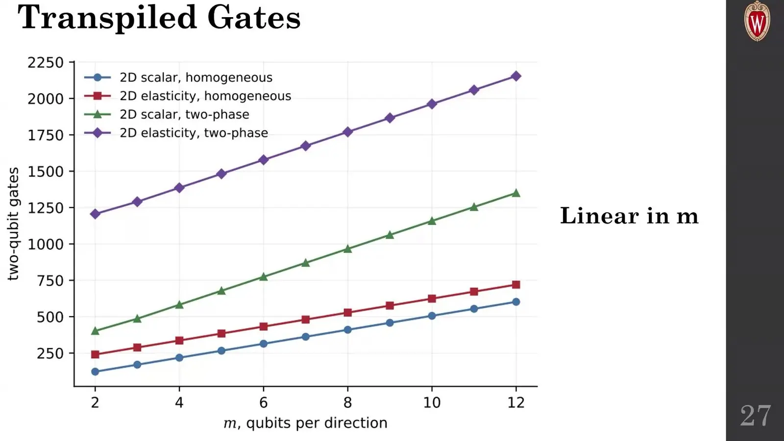
For the matrix that describes the grid, Suresh used the cyclic shift, which moves every row down by one and costs a known number of Toffoli gates. The matrix for Poisson’s equation, the simplest grid equation, on a looped grid in one dimension is then exactly three such pieces at any size, and in two dimensions it is nine. The shortcut needs regular grids and simple materials. Suresh agreed that a random mix of materials has no such pattern.

Kansas compiles solvers for flow and neutron transport

Esam El-Araby of the University of Kansas argued that trained circuits give poor accuracy and lose their training signal, while HHL leans on a step that noise easily spoils. So El-Araby built two other routes. The first, QSVD, uses classical maths to turn the grid’s matrix into an equal quantum step that standard tools can then build, and the second, QSVT, builds the solver from a sum of powers of the matrix.

Test cases ran from a wing to the Kansas Jayhawk mascot, plus neutron transport. On a 16 by 16 grid with 32 million shots, the first method reached fidelities of 0.83 to 0.85 on an emulated IBM chip with about 325,000 gates. A plain version of the second needed about 4.8 billion gates and gave no result. A tuned version fell to about 15.4 million.

Haiqu routes waves around obstacles at no extra gate cost

Maciej Koch-Janusz of Haiqu, a middleware company, presented joint work on equations that can be rewritten in the form of the Schrödinger equation. A grid with 2 to the power n points per side then fits in about n qubits, and Haiqu’s addition marks each obstacle and cancels its effect on the flow. Koch-Janusz said the gate count still grows only with the square of n.

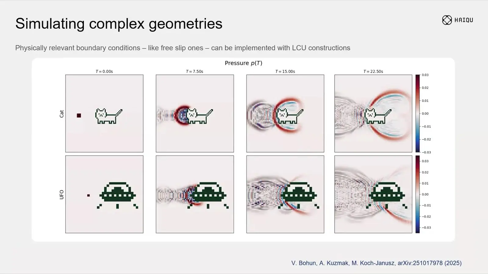
A demo scattered pressure waves around a pixel cat and a pixel UFO. The runs were on a simulator. Current hardware cannot run them. Koch-Janusz had no answer yet for nonlinear equations, and agreed that an airframe whose surface detail grows with the grid would lose the gain.

Solvers on real and simulated chips

Ten talks put solvers to work on IBM, IonQ and other chips, on a supercomputer and on simulators. The chip runs were small, and most of the good results came from simulators.

RPI and GE Aerospace benchmark Burgers’ equation on four IBM chips

Melvina Quartey, a doctoral student at Rensselaer Polytechnic Institute, presented a benchmark built with three researchers from GE Aerospace, one from Oak Ridge and Lucy Zhang of RPI. The rules are strict. The answer must be physical, the code must be ready for hardware and no classical answer may steer the quantum one, and the test case was Burgers’ equation, a simple model of flow that forms shocks.

One method turns Burgers’ equation exactly into the heat equation. Trimming its circuits cut depth and two-qubit gates by 75 percent. On hardware it ran on 8 grid points for six time steps on four IBM machines, and Quartey said every machine kept the right shape while the values drifted. Quartey called this method strong but narrow, and a second, lattice Boltzmann, the more general path.

Quanscient runs lattice Boltzmann on an 8 by 8 grid

Quartey, who worked at Quanscient as an intern this summer, also gave the company’s talk, standing in for Valtteri Lahtinen. Quanscient is based in Tampere and has about 40 staff. Its lattice Boltzmann method treats a fluid as packets of particles that hop and bump between grid cells. The hopping step is exact on a quantum computer, Quartey said, while the bumping step needs post-selection, keeping only the runs that came out right, which lowers the success rate.

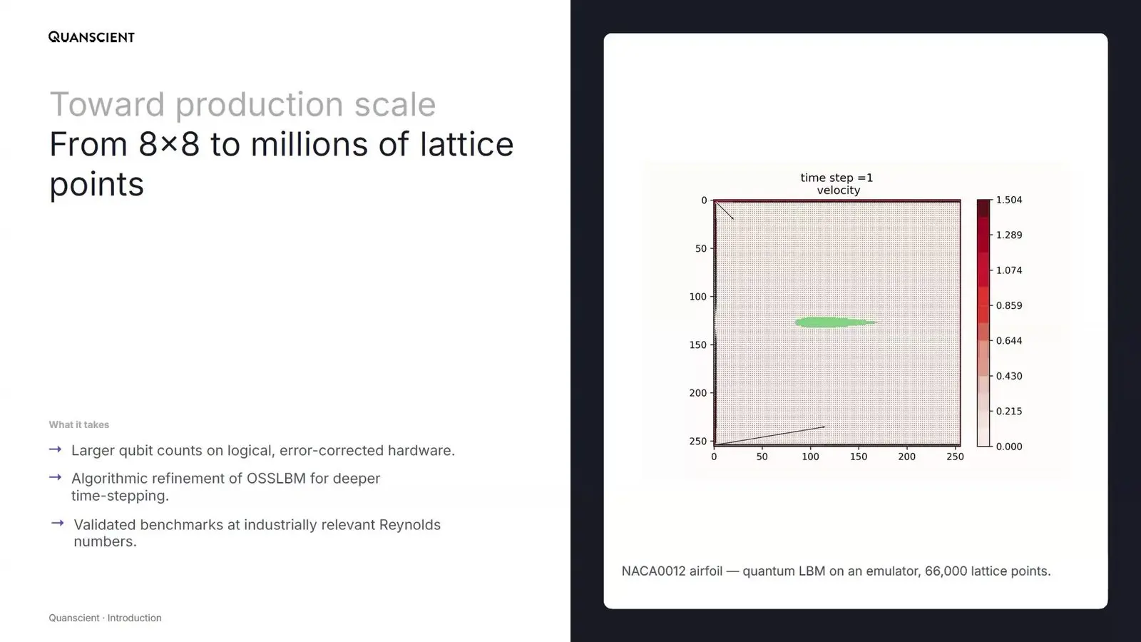
The team ran up to 15 time steps of flow past an obstacle on an 8 by 8 grid on real hardware, within what Quartey called reasonable error for noisy machines. A wing shape ran on an emulator at 66,000 grid points. Quartey said a full aircraft would need about 10 to the power 18 points, while 50 qubits can hold about 10 to the power 15.

Quanscient sweeps shots and gate noise in a tutorial

Oskari Kerppo of Quanscient closed a tutorial on tracking experiments in quantum workflows. Kerppo recapped the 8 by 8 run on a 156-qubit IBM Heron chip, which was checked cell by cell against a classical result and showed device error near 1 percent. A live notebook then ran a small flow problem on a local simulator.

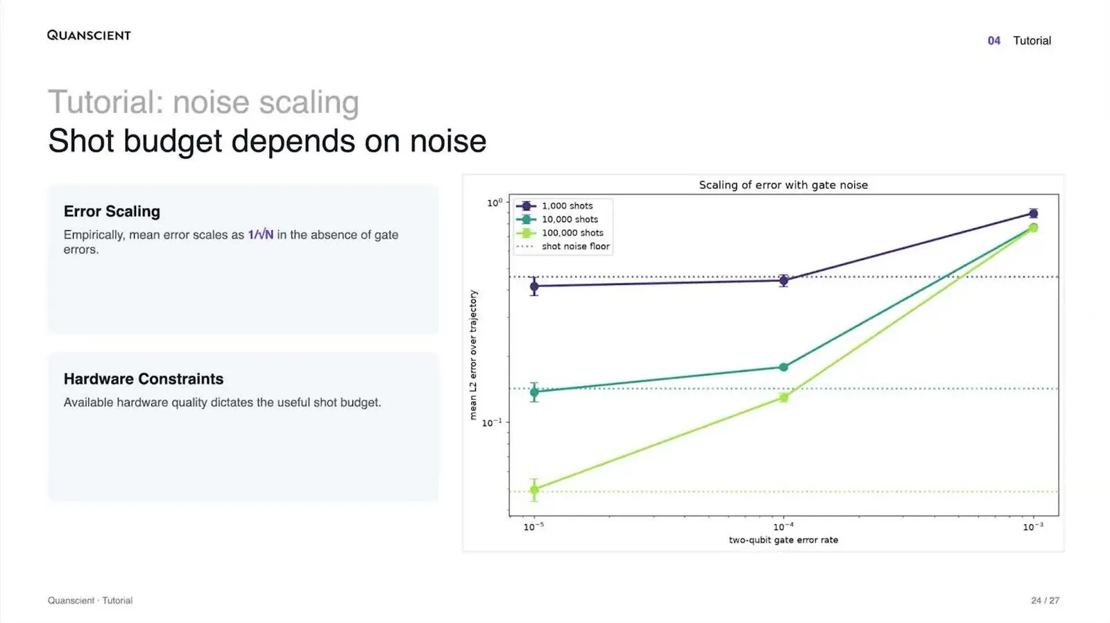
Kerppo then swept about 150 runs across three shot budgets and three gate error rates, and found that with gate errors of one in a thousand, 1,000 shots did as well as 100,000. More shots do not fix gate noise. Kerppo warned against adding qubits casually, because loading the state gets hard.

ColibriTD solves flow and option pricing with one trained circuit

Paolo Fittipaldi of ColibriTD, a Paris start-up of about 20 people, presented its solver H-DES, which is offered as a Qiskit function. H-DES writes the answer as a sum of known curves and uses the circuit’s measured odds as the weights. The same circuit gives the slopes as well.

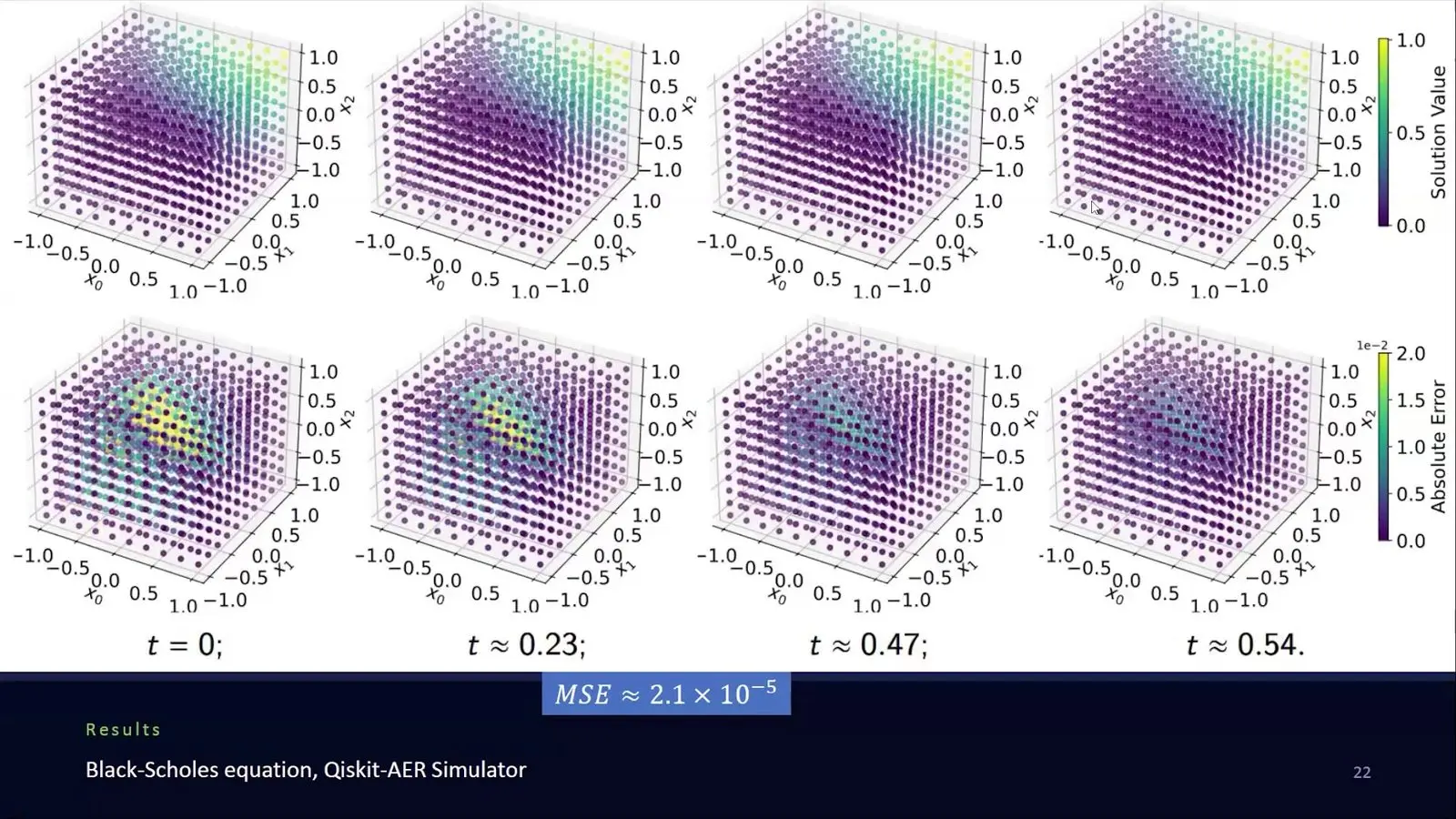
The first test was a simple fluid model on 70 qubits of IBM’s Fez chip, with about 30 minutes of machine time, and Fittipaldi said the results only partly agreed with the reference. The second test priced an option on three assets, which is a problem in four dimensions once time is counted. A noiseless run got the error very low. Read more about ColibriTD’s new funding.

Oak Ridge scales a variational linear solver on Frontier

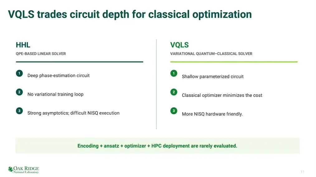
Kalyana Gottiparthi of Oak Ridge National Laboratory, a combustion scientist, stood in for Chao Lu and credited Lu with most of the work. Fluids already take 35 to 45 percent of Oak Ridge computing time. HHL asked for too many qubits on the simple flows the team tried, so they used a variational linear solver, which keeps a classical loop and suits noisy machines.

On one Frontier node, a new way of encoding the matrix reached a 256 by 256 grid in under 2,000 seconds, and one split ran more than 10,000 times faster per pass than the standard form. A flow between parallel plates passed 99 percent fidelity with four circuit layers. Gottiparthi said fidelities on their real engineering problems are still poor.

Florida Tech splits a power grid into pieces

Naveed Mahmud of the Florida Institute of Technology split a power grid into pieces, a method called diakoptics, and gave each piece to a small variational solver. Grid operators solve a large set of equations for the voltage at each node, and Mahmud said dense classical solvers scale as the cube of its size. A standard method keeps the voltages on the lines between pieces in step.

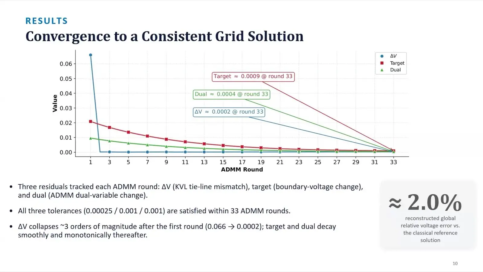
On the IEEE 9-bus test grid, after 33 rounds the mismatch on the tie lines fell from 0.066 to 0.0002, and voltages came within about 2 percent of a classical solve. The circuits were simulated on a graphics card. Asked what quantum adds once each piece is small, Mahmud said the pieces of large grids stay hard.

Vanderbilt poses stretching rubber as a circuit problem

Caglar Oskay of Vanderbilt University credited the postdoc Uditnarayan Kouskiya with the work. The topic was how rubber stretches. The right shape for a stretched solid is the one that stores the least energy, so that energy can be used as the cost that a trained circuit learns to bring down.

On a bar in one dimension with 3 qubits, the method matched the exact answer. Oskay said the cost grows only slowly with the size of the problem but with the square of the circuit’s depth, and how depth itself grows with size is still an open question. Until it is answered, nobody can price a large problem.

IonQ’s quantum cuts make a classical solver up to 14.6 percent faster

Willie Aboumrad of IonQ presented a paper that won a best-paper award in the QECS track. It works on one step inside LS-DYNA, a large engineering solver. A mesh of millions of points becomes a sparse matrix, and a careless order of its rows fills the matrix in until the later solve takes over the whole run. The classical fix hunts for balanced cuts of the mesh that set a good order.

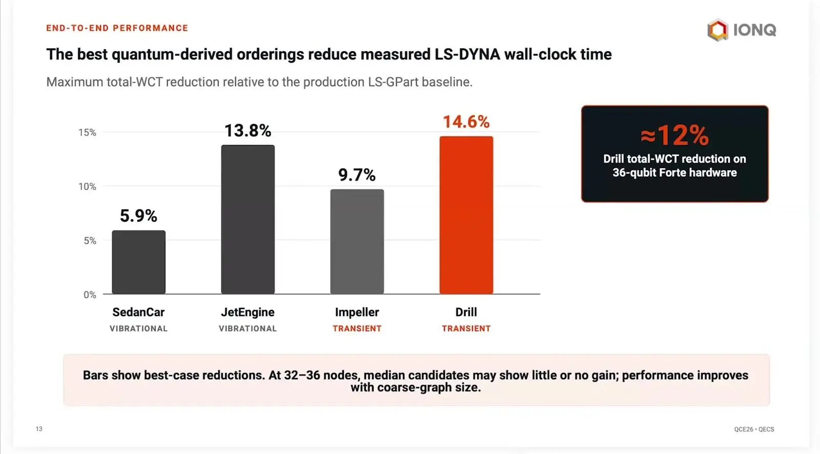
Aboumrad’s method shrinks the mesh until its graph fits on a present-day chip. A QAOA circuit with fixed angles then finds a balanced cut. The cut is lifted back to the full mesh for local touch-ups, and runs used IonQ’s 36-qubit Forte plus simulation out to 150 qubits, on meshes as large as a jet engine with 34.9 million points.

Against the production tool, the best cuts saved 5.9 percent of wall-clock time on a sedan and 14.6 percent on a drill. On Forte the drill saved about 12 percent. These are best-case picks. At 32 to 36 nodes the median candidate may show little or no gain, though gains grow as the shrunken graph gets larger.

Synopsys recovers the signs of electromagnetic fields on hardware

A Synopsys presenter showed work by Gautam Sharma and five colleagues on Maxwell’s equations, which govern electric and magnetic fields. The fields sit on a staggered grid. A step called Schrödingerisation recasts their evolution in a larger space where a quantum computer can simulate it. Because each grid point touches only its neighbours, the team broke the problem into pairs of qubits in a Bell basis, in place of the usual strings of single-qubit terms.

Measurements return only sizes, so the signs of the fields are lost. The team adds a fixed offset to one field to keep it positive, then compares sums and differences with every other field to win back all the signs. On hardware, a short simulated time and the Bell basis cut circuits from about 10,000 to 100,000 gates to within 1,000, on up to about 30 qubits. The signs survived.

IonQ and Ansys run 3D lattice Boltzmann on trapped ions

Jason Iaconis of IonQ presented work with colleagues from IonQ and Ansys, part of Synopsys. Their lattice Boltzmann method tracks dye carried along by a swirling flow in three dimensions, where the dye rides with the flow and does not change it. The density over 2 to the n grid points sits in n qubits. Each step is read out and loaded again. That keeps the circuits shallow.

A flow that varies from place to place would normally need a huge number of controlled turns of the qubits, one that doubles with each added qubit. Iaconis said a method called QPIXL cuts that sharply for smooth fields such as this swirl. Tensor networks help load and read the densities. After one step, circuits of hundreds of CNOT gates matched the ideal density with a fidelity of 0.96, or 0.97 after smoothing, and the team ran six time steps on IonQ’s Forte and a barium test system.

Iaconis called nonlinear flow the open challenge. Reloading the state after every step keeps the circuits short, but it also means that every step must pay again for getting data in and out.

Tensor networks, quantum-ready and classical today

A tensor network squeezes a large grid into a chain of small linked blocks by keeping only its strongest links. It borrows the maths of quantum states, runs on ordinary computers and graphics cards today, and could be moved onto quantum machines later if they ever pay. Four talks made the case for it.

AWE expects no single winner

Claudia Clarke of AWE expects any quantum gain in fluid dynamics to arrive as raw speed, and spoke for joint work with Callum Duncan and Dean Johnstone of Aegiq. AWE supports the UK’s sea-based nuclear deterrent and, since full-scale tests of the old kind are no longer possible, relies on modelling. Its quantum team is about 10 strong.

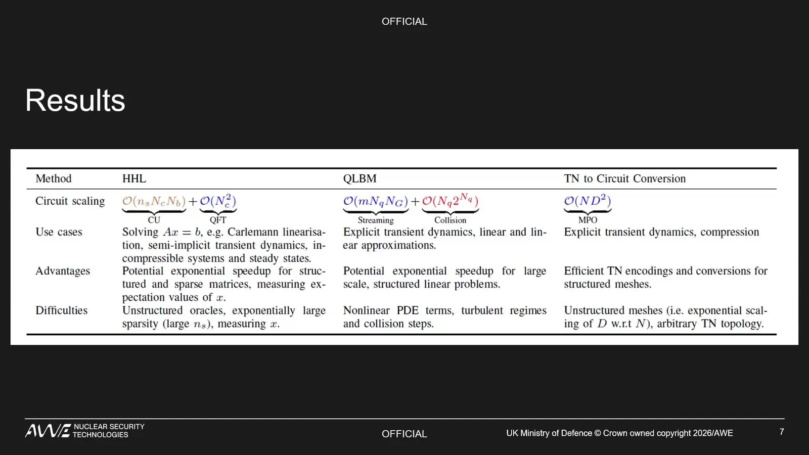
Clarke weighed three routes on one table. Lattice Boltzmann mirrors a familiar classical method but has no clear path to nonlinear flow, HHL needs sparse matrices, and tensor networks already run on classical hardware but can blow up on irregular meshes. Clarke concluded there is unlikely to be one winner.

AWE squeezes plasma simulation into tensor networks

Preetma Soin of AWE presented work by Ryan Connor, a former student of Soin’s, with Andrew Daley and Callum Duncan. Plasma is the charged gas in fusion machines and lasers. Codes that model it push simulated particles across a grid, and Connor’s method splits that grid into finer and finer length scales and squeezes it into a chain of small tensors.

Connor’s runs of two standard plasma cases matched a run Soin made in a classical particle-in-cell code. Soin said scaling is still the open issue.

Oxford keeps a shock front sharp

Ryan Connor of the University of Oxford, working with Andrew Daley, used tensor networks for compressible flow, the fast kind that forms shocks. Shocks set off false ripples, and the usual fix needs a square root and an absolute value that tensor networks cannot compute directly. Connor rebuilds that fix from sampled rows and columns.

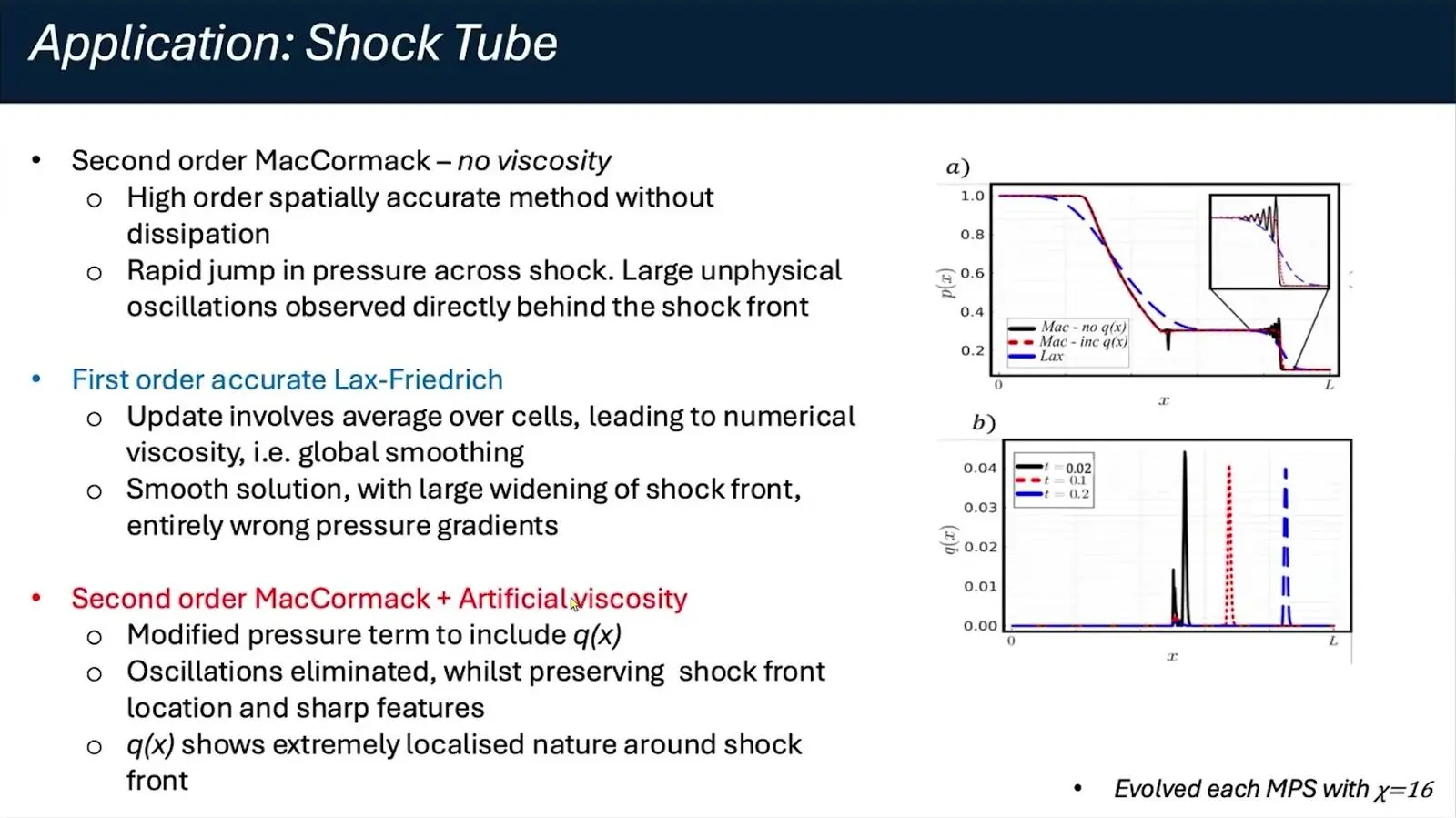
On the Sod shock tube, a standard test, one classical scheme rang with false ripples behind the front and another smeared the front out over many cells. Connor’s version kept a sharp, clean shock with small blocks. Connor said any such tensor chain can be written as a quantum circuit.

Aegiq pitches memory savings within two years

Callum Duncan of Aegiq, which builds quantum computers that run on light in Sheffield, writes what Aegiq calls quantum-ready methods. Most are tensor networks. They run on graphics cards now and could move to quantum hardware later, so the pitch to customers is a gain within two years, such as 100 terabytes cut to 100 kilobytes, and maybe more later. Duncan prefers that to near-term trained circuits.

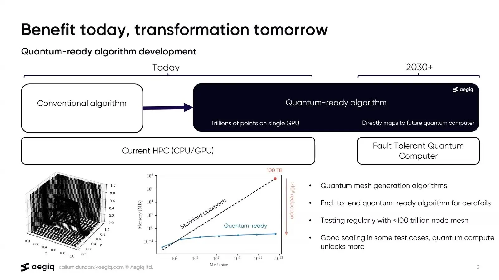
Aegiq’s projects include a wing simulation with BAE Systems and NVIDIA, a meshless method with MBDA and the squeezing of turbulence data from the Frontier supercomputer. The next target, set by BAE Systems, is NASA’s Common Research Model aircraft. Duncan planned a full demo by the end of April.

Where the advantage would come from

Three sessions asked where a real quantum gain in this field might first appear. They also asked how anyone would know.

IBM sorts its solvers by how nonlinear the flow is

Mykhaylo Zayats of IBM Research in Dublin sorted the team’s work by how nonlinear the equations are. Linear problems get solvers of their own. Mildly nonlinear ones get the Carleman method. It turns a nonlinear system into a larger linear one. Strongly nonlinear ones, such as the Navier-Stokes equations that govern real fluid flow, get a new solver that Zayats’s team built on the Kolmogorov equation.

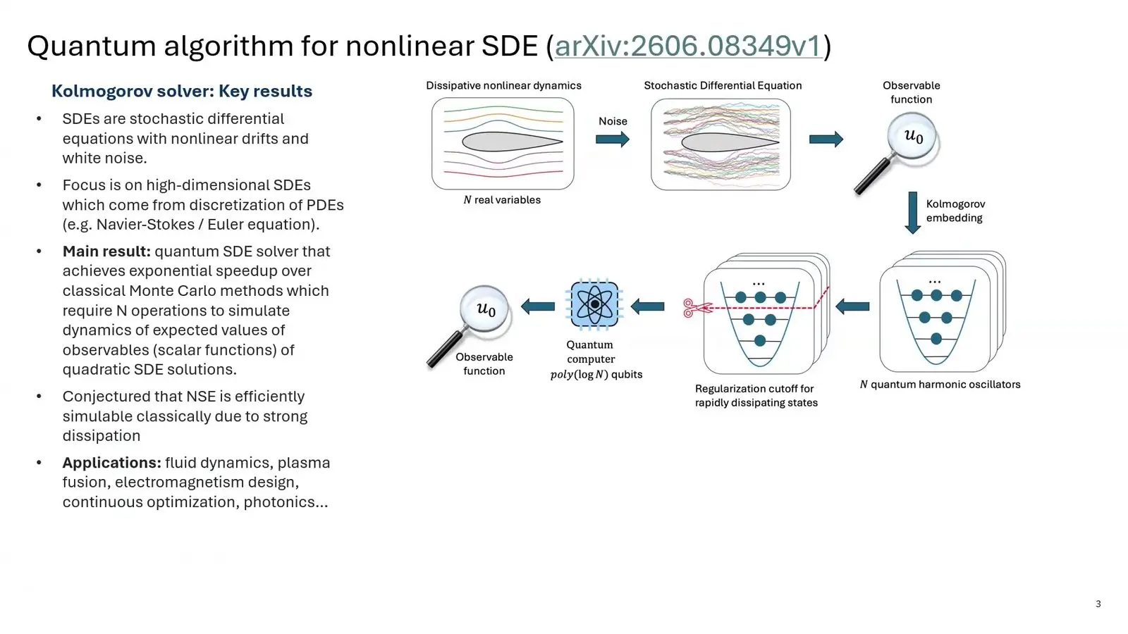
That solver adds noise to the equations and tracks a single number from the answer through an equation that is linear. Zayats said its run time grows only slowly with problem size, and colleagues hope for a prototype on current hardware within months. On the panel Zayats asked for full cost counts. Those must include loading and readout.

Cascade Quantum reads out coefficients instead of fields

Sonika Johri said Cascade Quantum spent a couple of years in stealth and had only begun to speak in public the month before. Its first product is Red Cedar, a learning platform. Johri argued that learning methods are underused for hard equations on quantum machines, given what neural networks have done on classical ones.

Because loading and reading out data can wipe out any gain, Johri suggested using the quantum computer to learn a few numbers that describe a solution and then working them out on a classical machine. Johri expects an advantage where a problem is simple to state and read out but hard to solve.

The panel declines to pick a winner

Andrew Gallo of GE Aerospace Research moderated a panel with Duncan, Quartey, Zayats, Johri and Amir Shehata of Oak Ridge. Shehata described openQSE, a group agreeing on software layers from the application down to the device, which has grown from two members, Oak Ridge and IonQ, to about 34. Duncan bet on the huge direct simulations engineers use to check their models. Quartey suggested pulling out single numbers such as drag and lift.

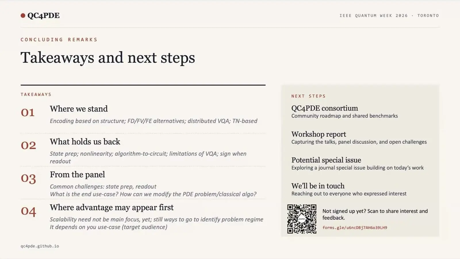
An audience member said nobody had mentioned preconditioning, a standard trick for making equations easier to solve, all day, and Duncan doubted that linear solvers will amount to much. Duncan ended by saying the field is not ready to pick winners. The organisers listed loading, nonlinearity and readout as the main hurdles. Next come a QC4PDE group and a workshop report.

The bill for the doors

Brightskies Technologies of Alexandria ran a two-part class for software engineers on how to turn a classical solver into a quantum one. The second part set out the clearest prices in this guide. Two more talks added to the bill.

Brightskies lays the groundwork

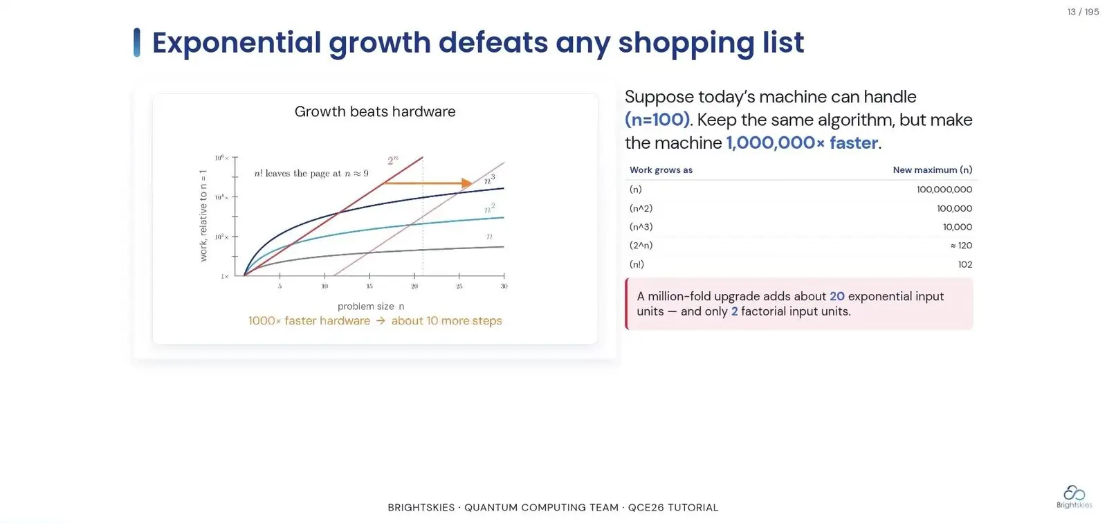
Mahmoud Elkarargy, a senior engineer who leads the technical work of the quantum team at Brightskies, opened the class with a colleague. A chart showed that for work that grows very fast with size, a machine a million times quicker only lifts the size you can solve from 100 to about 102. Quantum is a speed-up only when the problem’s shape fits, Elkarargy said.

Elkarargy then built up from a single coin-flip circuit to a two-player game, Grover search and Shor’s algorithm on the number 15. This first session never reached the heat equation. It set out what a quantum speed-up can and cannot be.

Brightskies prices the heat equation

Two Brightskies presenters finished the class on the heat equation in one dimension, using eleven quantum building blocks from the team’s QCE26 paper and its free HelloQuantum code. Loading any 1,024 numbers took about 2,026 CNOT gates. Worse, the data goes back to the classical side after each step, so it must be loaded again every time.

On an ideal simulator with 100,000 shots per step, a kernel called QSM kept a relative error of about 2 percent, while HHL’s spare qubit succeeded only once in 6,700 runs. Reading the answer out cost even more. Rebuilding the full 128-point field to about 1 percent took about 1.28 million shots, against about 10,000 for one average. Compiled for IBM’s Sherbrooke chip, one time step needed about 30,800 two-qubit gates and would last 18,100 microseconds against a qubit memory of 170, which the team called 106 times too long. So for this problem the solve cost far more than the loading.

Yokohama finds where QSVT overtakes Trotter on the heat equation

Taito Mizutani of Yokohama National University presented work with four co-authors from Japan and San Diego. Most grid equations change over time in a way a quantum computer cannot apply as it stands, because they let the total fade or grow while quantum motion keeps it fixed. So a step called Schrödingerisation adds one more variable, and that turns them into the plain kind of motion a quantum computer can run. QSVT then puts a chosen polynomial to work on a matrix tucked inside a larger quantum step. That trick is called block encoding.

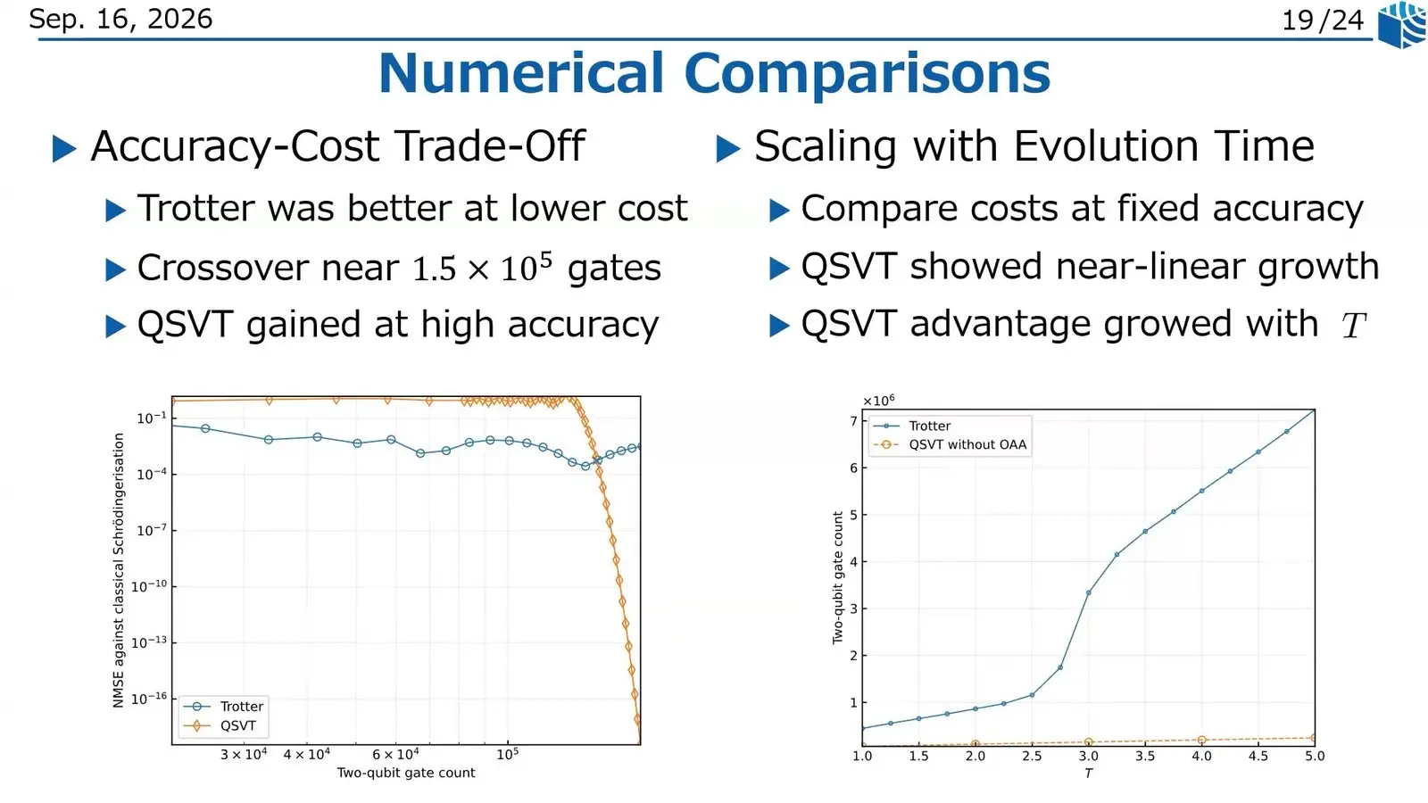
Mizutani built that block encoding for the heat equation by hand, with cyclic shift circuits for the grid. In noiseless simulation QSVT was worse at low gate counts. Its error fell steeply as the polynomial grew, and beyond about 150,000 two-qubit gates it beat a Trotter method, the usual approach of splitting the evolution into short steps. At fixed accuracy its cost grew roughly in line with the evolution time, while Trotter’s grew faster.

Brightskies’ paper puts eleven heat solvers side by side

Mahmoud Elkarargy of Brightskies Technologies gave the team’s paper the day before the class, with three co-authors. Published error figures cannot be compared, Elkarargy argued, because each team uses its own code, its own shot budget and its own guess about the hardware. So the team ran eleven solvers on one heat equation.

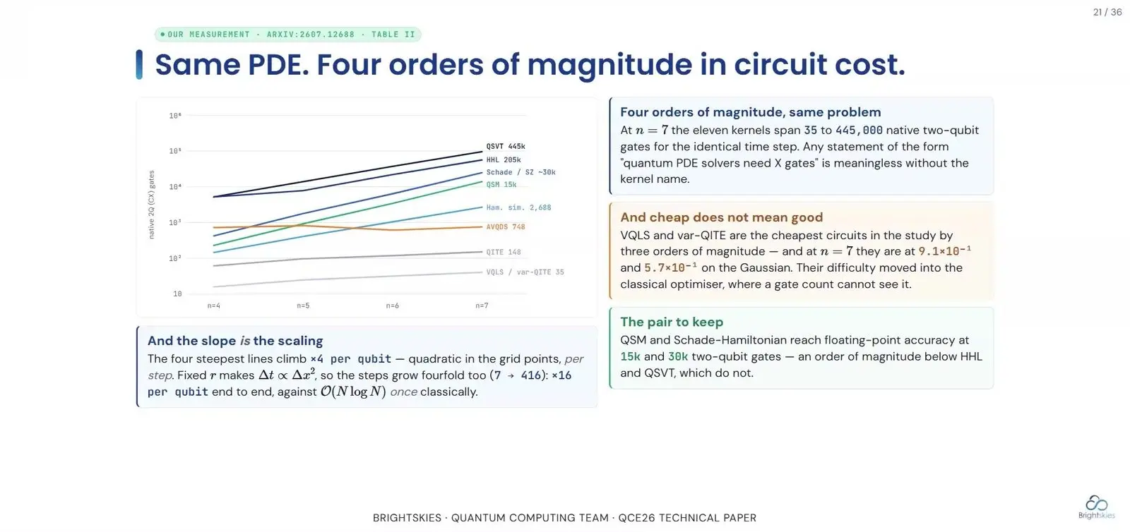
At seven qubits, one time step needed anywhere from 35 to 445,000 two-qubit gates. On exact simulation two methods matched the classical answer to machine precision, while with sampling their error rose to about 2 percent. Three unrelated solvers shared almost the same error on smooth profiles, which led the team to split the error into scale and direction, since quantum states are normalised and lose the overall size of the answer. On a square pulse the scale mismatch made up 94 to 100 percent of the error. On a Gaussian it was about 23 percent.

What it means for quantum CFD buyers

For an engineer deciding where to spend, the order of work is clear. A claimed quantum speed-up on a flow problem means little until loading, readout and circuit depth are priced from end to end, as Brightskies did for one heat equation. Tensor-network codes already run on classical machines, and their backers say later quantum hardware could inherit them.

For the maths, see our guide to the linear algebra behind it. Every chip result in this guide stayed at toy size, so quantum solvers for these equations look good on paper and are still unproven in practice, however neat the algorithms behind them. Suresh warned about the first door on day one. By Thursday the room itself carried the biggest bill.