Quantum benchmarking at QCE26 turned into an audit

This guide follows 55 talks on quantum benchmarking, error mitigation and classical simulation at IEEE Quantum Week 2026 in Toronto. The best results came from the people who check quantum claims.

On Monday 14 September, in a workshop in Room 718A of the Metro Toronto Convention Centre, Salvatore Mandrà of Google Quantum AI described a classical simulation of a 56-qubit run by Quantinuum, a rival firm. It kept pace with the quantum machine. Mandrà said it also showed up errors in Quantinuum’s first published data, which the firm later revised. An ordinary computer had checked a quantum one and found a fault in its record. For quantum benchmarking, the job of measuring what these machines can do, the roles had been reversed.

Every claim about a quantum computer rests on a measurement, and today’s machines are noisy. Each gate has a small chance of going wrong, qubits slowly lose their state and readout sometimes returns the wrong bit, so the longer a circuit runs, the more its answer fades toward random noise. Quantum benchmarking measures how bad this is. Some tests take the machine part by part, as with the error rate of one gate, while others run whole circuits and boil the result down to one score. Each choice of circuit and score favours some machines over others, which is why benchmarks are argued over so fiercely.

Error mitigation tries to clean up the answer without the full machinery of error correction, which is still being built. It runs a circuit many times in altered forms and uses classical sums to guess what a noise-free machine would have returned, so its price is paid in extra runs. A poor fit can even return values that are physically impossible.

The hardest question is whether a machine has done anything a classical computer could not. The field calls that quantum advantage. Writing down the full state of n qubits takes 2 to the power n numbers, so a few dozen qubits outgrow the memory of the largest supercomputers. But classical methods rarely need the full state. Tensor networks break a big state into many small linked pieces and do well when the qubits are not too tangled. Since Google’s random-circuit test of 2019, many of the best-known claims of advantage have drawn a classical reply of this kind.

The 55 talks followed here, from the conference also known as QCE26, suggest who now holds the pen on that question. The auditors do. They are the classical simulators and sceptical benchmarkers who test each claim as it appears, and a quantum claim now stands only once they have tried to wash it out and failed.

The quantum side had its say, and it brought hardware. Hayk Tepanyan of BlueQubit presented a paper on peaked circuits that won a best-paper award in the QALG track. Its hardest instance ran on 56 qubits of Quantinuum’s H2 machine. Harry Buhrman of Quantinuum argued that better hardware leads first to discovery and only later to industrial use, a fair answer to anyone who demands a business case from every experiment. Some of these claims may well hold up. They were made, all the same, on ground the auditors had chosen.

The auditors made their case all week. Joseph Tindall of the Flatiron Institute was the most forceful of them. Belief propagation, the method Tindall uses, matched or beat an IBM test from 2023 and a D-Wave result, both billed at the time as beyond classical reach. Glen Evenbly of NVIDIA showed how to correct the method loop by loop, and Dominik Köster of OTH Regensburg showed error mitigation giving 1.16 for a value that cannot pass 1. Köster then checked 83 papers and found their statistics the weakest part. Siddarth Shinde of Northwestern showed that adding price changes which machine looks best.

Yet the deeper change is in who gets to check. If outsiders are to do the checking, they need something to check. Several teams learned useful models of real hardware from ordinary run data, which makes raw shots worth more than any summary score. On the Wednesday, Alessandro Cosentino of the Unitary Foundation found that most benchmarks in a public store of results largely measure one shared noise budget. On the Thursday, the standards bodies described efforts to sort benchmarks and track error-correction claims, and a questioner from the floor said vendor numbers still cannot be checked by anyone outside. The audit culture the simulators built has yet to reach the spec sheet.

Classical simulators answer the advantage claims

Seven talks came from people whose job is to follow quantum machines with ordinary ones. Most spoke in a Monday workshop on simulation, and their message was that the gap is narrower than the headlines said.

Rescaled matrix product states catch a Quantinuum error

Salvatore Mandrà of Google Quantum AI, one of the workshop organisers, took on Quantinuum’s H2 experiment published in Nature in 2026. It ran a standard magnet model on a 7 by 8 grid for 20 steps near a phase change. Quantinuum had judged that a chain-shaped tensor network, called a matrix product state, would need so much memory that classical methods could not pass eight of those steps. Mandrà set out to test that.

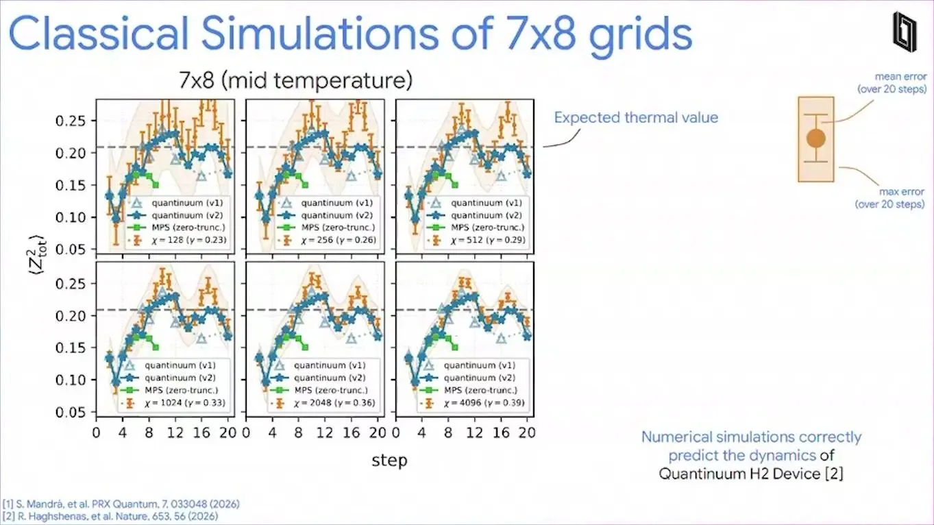
Mandrà’s trick multiplies the rough result by the simulation’s own fidelity raised to a fitted power, on the view that each cut throws away something close to random noise. Mandrà fitted the power from exact runs on grids up to 6 by 6. The error bars held against an exact 6 by 8 simulation.

On the 56-qubit grid the method ran in about two days on one A100 graphics card. Mandrà said it showed Quantinuum’s first published data were wrong, and that the company’s revised version now agrees with their curves to below 2 percent. Larger grids were inconclusive. Mandrà said the method works because of this model’s physics and cannot work in general.

The same result, shown again on Thursday

Mandrà gave the talk a second time on the Thursday, in HPE’s workshop on quantum supercomputing. The questions from the floor added new material. Asked where hard tests lie, Mandrà cited Google colleagues who argue this magnet problem would show quantum advantage on an error-corrected machine with only 121 logical qubits. That compares with about 10,000 for the FeMoco chemistry test.

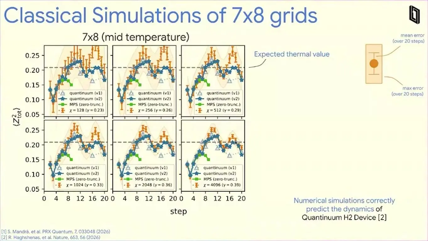
A questioner from Quantinuum suggested running the same error estimate on the quantum machine. Mandrà welcomed the idea. Mandrà again called the larger grids, 8 by 8 to 11 by 11, inconclusive, and said their apparent agreement could be a fluke.

Belief propagation beats IBM and D-Wave claims

Joseph Tindall of the Flatiron Institute recalled their simulation of IBM’s 2023 heavy-hex test. It got errors of about one in a million on a large measured value, while the quantum computer sat near one in a hundred. Their tool is belief propagation. It passes messages along each link of a tensor network until they settle, and so turns one big costly sum into a lot of cheap local ones.

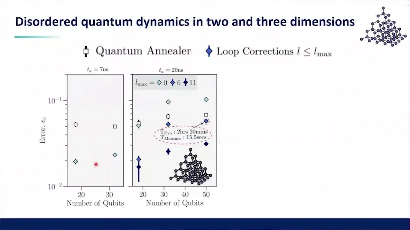
Their hardest test was D-Wave’s 2025 Science paper on annealing spin glasses, which claimed results beyond classical reach. Tindall said plain belief propagation already beats the annealer for short anneals. Longer ones took more work. Extra terms then brought the error well below the annealer’s on a 3D lattice, and their method’s cost grows as the sixth power of the entanglement it keeps, against the 29th power the paper had claimed.

The work runs in an open-source package that supports graphics cards. Tindall reported runs on about 12 NVIDIA H200 cards. One chemistry sampling run took 1.9 seconds on a graphics card, against 110 seconds on an ordinary processor, which shows how much of this race now turns on hardware built for AI.

Loop corrections close the gap further

Glen Evenbly had joined NVIDIA’s cuQuantum team about a week earlier, after leaving AWS. Evenbly framed the field as an arms race. Experiments are built to defeat classical methods, and classical methods are built to catch them, and belief propagation is exact on networks without closed loops but a few percent off with them.

Evenbly’s loop series adds back corrections for closed loops in order of size, smallest first. On a standard test state, plain belief propagation was within 0.2 percent of the exact answer. Corrections cut that error by several orders of magnitude. Evenbly said states with several equally good ground states remain a problem, since the method picks one and the others show up only late in the series.

Majorana propagation for electrons

Matteo D’Anna of ETH Zürich, working with colleagues at ETH and EPFL, carried a method called Pauli propagation over to electrons. It follows the measured value instead of the state. It drops small terms as it goes and tracks how much it threw away, and on one measure from a hardware run their classical answers agreed with each other but sat below the device. With only about 1 percent thrown away, D’Anna judged the classical answer the likelier to be right.

For a second measure every classical curve matched the hardware. Yet the classical truncation had thrown away about 90 percent of the operator’s norm, its measure of size, and a match built on so little of it proves nothing, however neat the curves look. D’Anna’s advice was to tighten the cuts step by step and watch both the answer and the share that was dropped.

NVIDIA’s faster simulators and small AI models

Taylor Lee Patti, who manages the Quantum Simulation and AI Research Group at NVIDIA, opened the simulation workshop. Their group draws errors up front and reuses each built state for many shots, so a noisy run no longer means building the state from scratch every time. Patti quoted a speed-up of 200 to 1,000 times. A year before it was 30 or 40.

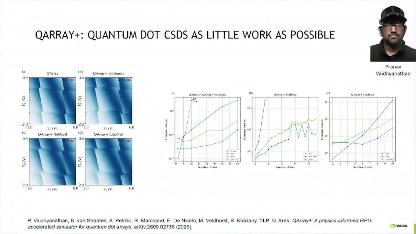
Their favourite tool is the Fourier neural operator. It is a network that learns a physics equation, and Patti said it runs about a million times faster than a solver. A small network of about a thousand settings, trained on about a thousand runs of a field solver, matched the solver’s own accuracy for qubit design, Patti said.

The simulation workshop ended split on advantage

Dmitry Lyakh of NVIDIA, one of the organisers, led the open debate that closed the two-day workshop on simulation on the Tuesday. It ended split. One person in the room, who once co-wrote a challenge to Google’s supremacy claim, now expects a niche advantage soon. Others doubted that a quantum computer can beat classical methods on classical cost functions, some 30 years after Shor.

An experimentalist thought quantum dynamics would come first. That, the experimentalist warned, needs a kind of trust that no one can check on a laptop. The wish list was long, and it ran from spotting the symmetries of a lattice by machine to cavity modes for GKP qubits, as built by Nord Quantique, where each mode may need about 200 levels.

Claims of quantum advantage

Five talks argued for a quantum edge, by showing hardware results or by firming up the theory behind them. They made that case in a week when classical simulators were busy answering earlier claims.

Peaked circuits on 56 qubits

Hayk Tepanyan, co-founder and chief technology officer of BlueQubit, presented a paper that won a best-paper award in the QALG track. The programme lists Nicholas Sherman, Hrant Gharibyan, Zuhair Mullath, Vincent Su, Tepanyan and Yuxuan Zhang. A peaked circuit looks almost random but hides one bit string with a high chance of turning up, so a quantum machine can find it fast and anyone can check the answer. That pairing of hard to find and easy to check is the appeal.

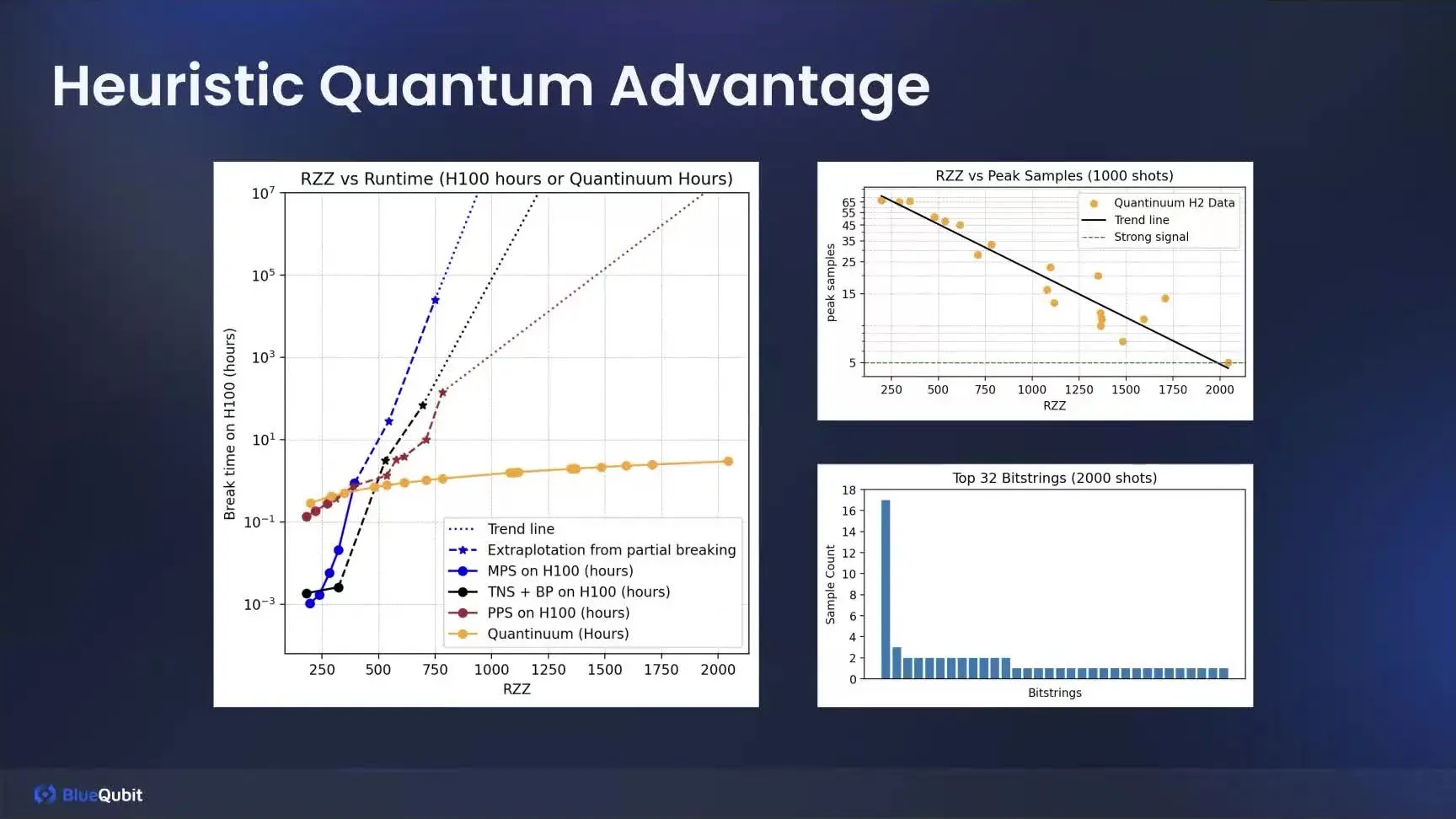
The hard instance ran on Quantinuum’s H2 with 56 qubits and 2,000 two-qubit gates. Tepanyan said the machine finds the peak in minutes to hours, while time on top graphics cards for the same circuits climbs by orders of magnitude. An IBM note from April 2026 tries to peel away the hidden structure. Tepanyan said a generic run of that attack stalls or runs out of memory on about 90 percent of a few hundred circuits, while a hand-tuned attack can break a single circuit in a week or two.

Wiring decides whether noisy circuits stay hard

Leonardo Placidi of Quantinuum presented work with Enrico Rinaldi, Keisuke Fujii and Chen-Yu Liu on IQP circuits, whose gates can run in any order. Theory says sampling from them is hard for classical computers. Noise weakens that guarantee. On chips where qubits only talk to neighbours, extra routing steps make circuits deeper and noisier.

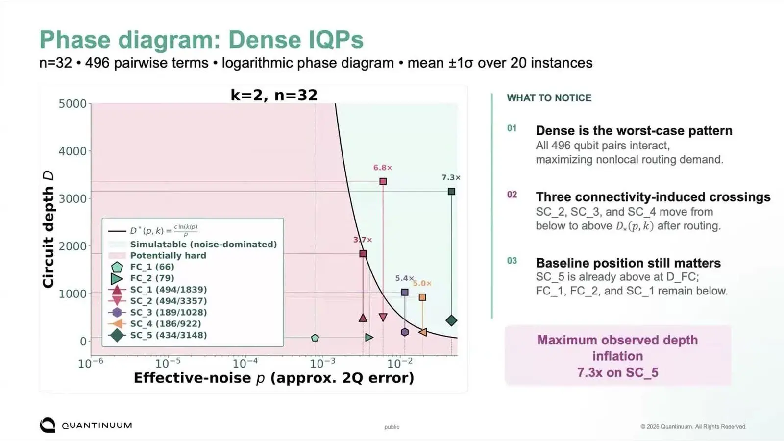
Placidi compared seven layouts, from machines where every qubit links to every other to a 127-qubit heavy-hex map. Dense 32-qubit circuits grew up to 7.3 times deeper after routing on a sparse layout, and three sparse layouts crossed into the zone classical computers can simulate only after that routing. Both fully linked machines stayed hard. So a claim can slip with no new classical method at all.

A step toward proving boson sampling is hard

Bin Cheng of the National University of Singapore presented work with Fei Meng, Jianan Li and Man-Hong Yung on boson sampling, an experiment that sends photons through a maze of beam splitters. Its claim to classical hardness rests on two unproven pieces. Cheng tackled one, the claim that a key quantity of a random matrix rarely comes out tiny.

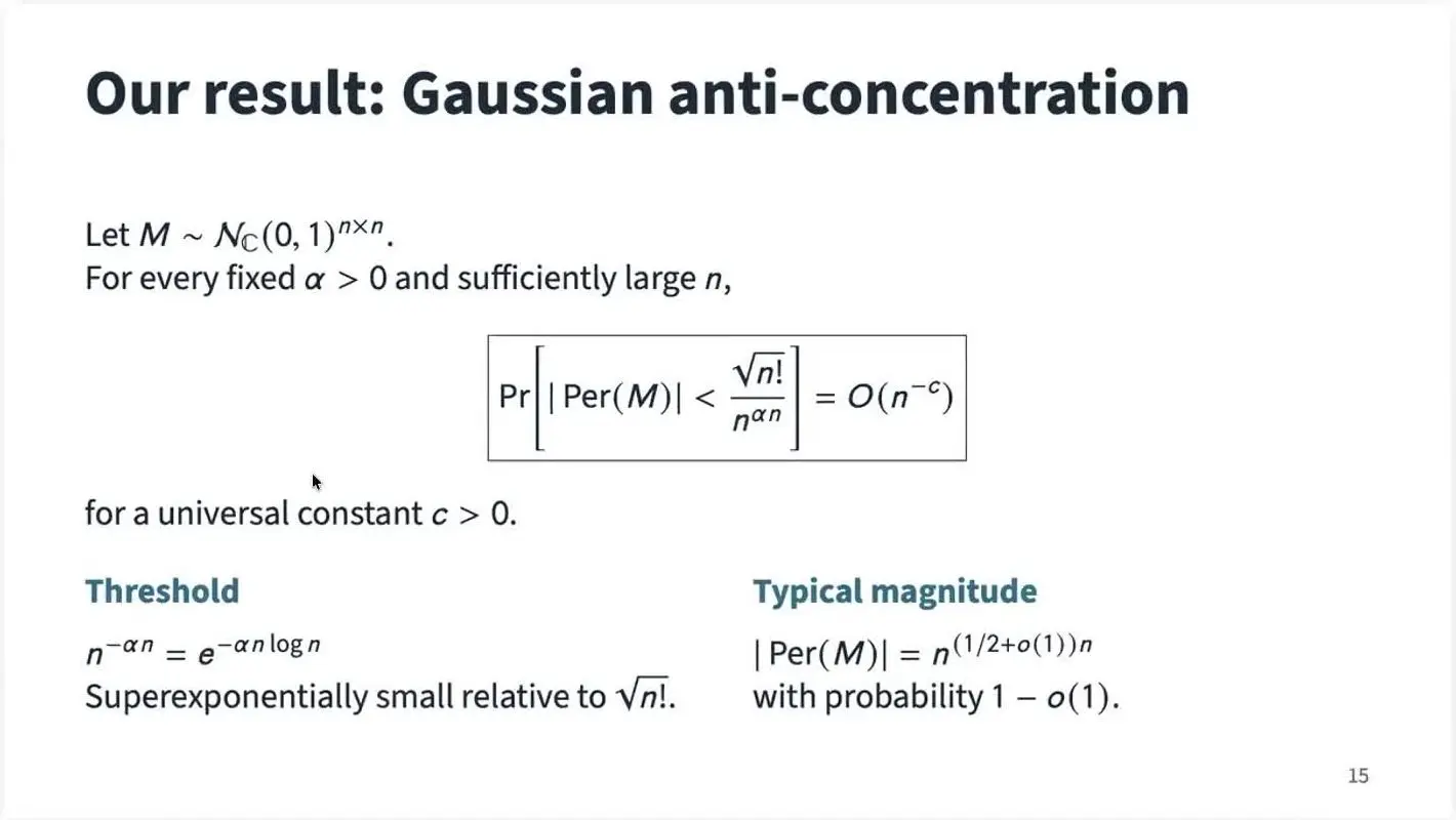
Their new bound proves a weaker form of that claim, which Cheng said still falls short of the strength the full conjecture needs. Cheng also said a 2026 note by other authors claims the full bound. Cheng had only checked it with a chatbot.

Complement sampling and a bottom-up route

Harry Buhrman of Quantinuum argued that better hardware leads first to discovery and only later to industrial use. Buhrman opened with van Leeuwenhoek’s microscope of 1674. Their first example was complement sampling. Given a sample from a hidden set holding half of all strings of a given length, a classical player can barely beat a coin flip at naming a string outside it, while a short quantum circuit does it reliably.

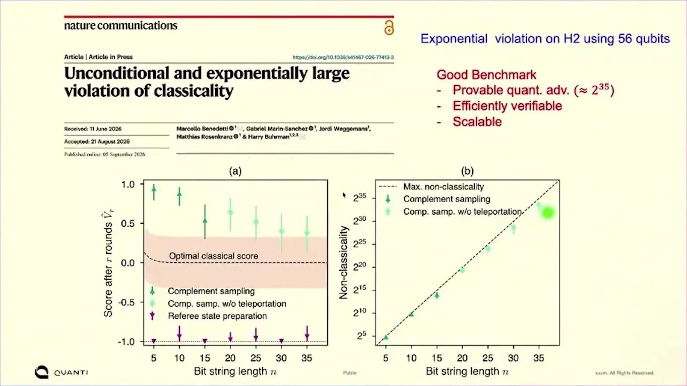
On H2, in a Nature Communications paper out on 5 September 2026, the team reached strings 35 bits long on 56 qubits. Their second example was a white paper with SoftBank on phone-call networks, in which the values a quantum method can estimate told fraudsters from normal callers where the usual counts did not. A questioner said bottom-up tests have run for 20 years with no practical gain. Buhrman’s reply was short. Top-down work, Buhrman said, has shown none yet either.

Complement sampling tracked the theory line to 35 bits

Harry Buhrman, chief scientist for algorithms at Quantinuum and a professor at the University of Amsterdam, gave a first version of this case on the Wednesday, in a workshop on accelerated quantum supercomputing. The core was the same. A single Grover step, a standard move in quantum search, turns a superposition over the hidden half of all strings into a sample from the other half. On H2 the result followed the theory line up to 35-bit strings, which Buhrman put at about 2 to the 35th and called easy to verify.

The team found sets that are easy to prepare with help from ChatGPT. Buhrman said the field is in a phase of discovery that will come well before industrial use, and urged that an algorithm be judged on typical cases and not on the hardest one. Then came a further plan. It is to simulate laser-induced superconductivity in yttrium barium copper oxide with an extended Fermi-Hubbard model.

Error mitigation under audit

Error mitigation is the workhorse of today’s noisy machines. Nine talks tested its limits or pushed it further, and one found a mitigated value that physics forbids.

A parity of 1.16, which cannot happen

Dominik Köster of OTH Regensburg, with Wolfgang Mauerer, opened a Wednesday benchmarking block with a result that was too good. Zero-noise extrapolation runs a circuit at raised noise levels and draws a line back to zero noise. On a four-qubit circuit on IQM’s Euro-Q-Exa machine, the raw value was 0.59, the corrected value 1.16 and the true value 0.96. A parity can never exceed 1.

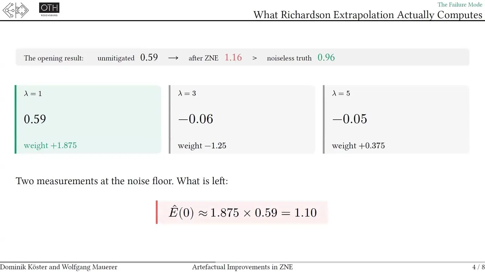
Köster traced this to the fixed weights of the fit. When the two noisier runs sit at the noise floor, the answer collapses to 1.875 times the first reading, which looks like a real gain but is an artefact of the sums. Their check applies the same weights to every outcome and adds up the negative parts. It costs nothing extra. Over 30 repeats it read 0.02 for a faithful case and 0.27 for the overshoot.

Most error-mitigation papers skip the statistics

On the Friday Köster went further. Köster had tried to rebuild a published four-qubit result and could not, because the IBM machines had been retired and the paper left out key settings. So Köster scored 83 recent error-mitigation papers on eight questions, and found statistical tests and any account of drift the thinnest parts.

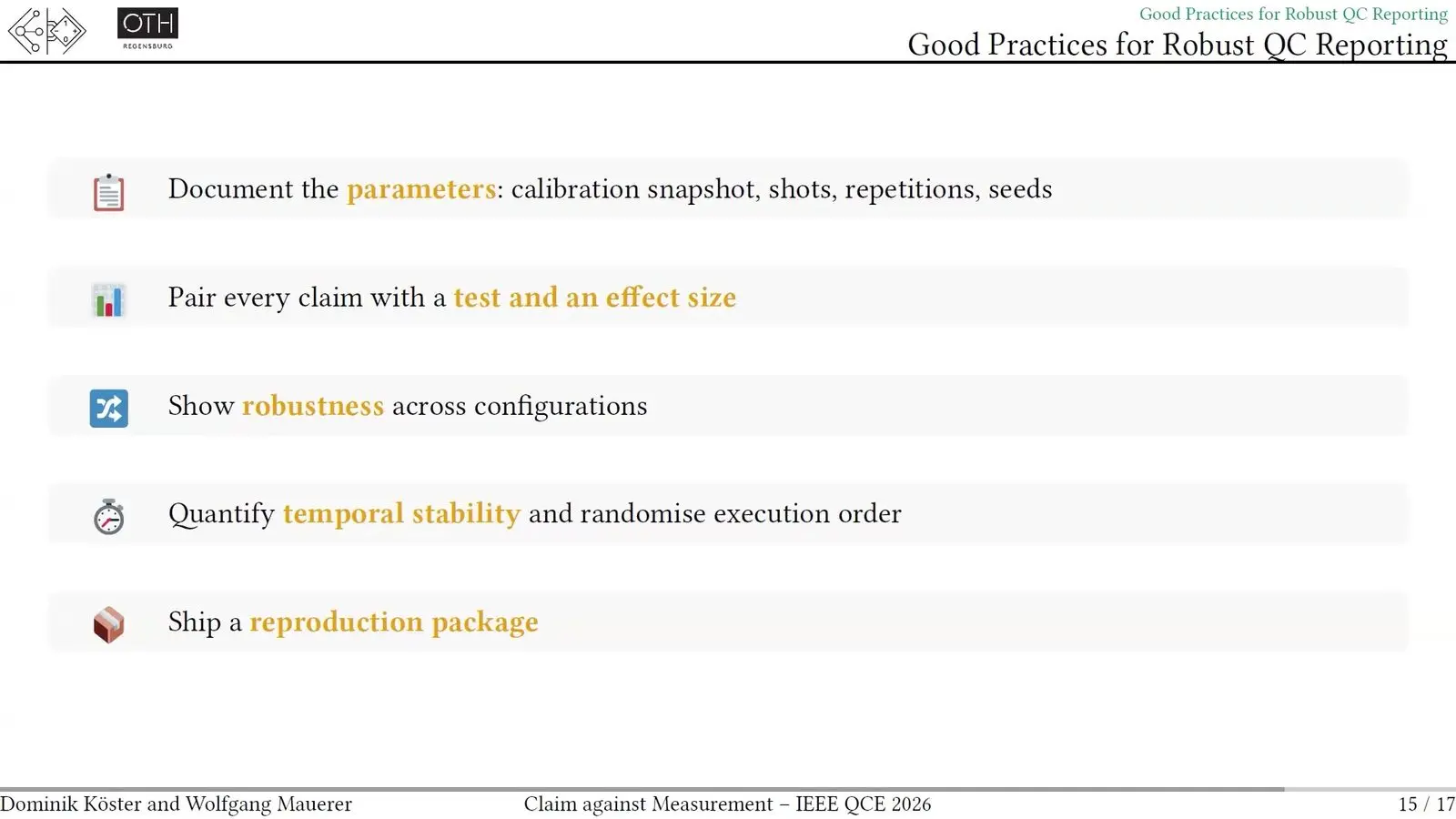
Their own runs showed why that matters. Some circuits needed more than 10 repeats to reach a fair test, while papers often stop at 5 or 10. Thirty repeats taken every half hour counted as only about 1.8 independent measurements, because the machine itself changes over time and runs taken close together tend to agree. The timing of a measurement mattered most. Köster put 55 percent of the spread down to when a measurement was taken, and their checklist asks authors to record their shots, repeats and seeds and to ship a package that rebuilds the figures.

Unblurring noisy answers

Phat Thanh Tran of Florida State University presented work with Xiuwen Liu. Wrong answers tend to cluster near the right one. So a string one bit away from the target is more likely than one two bits away, and their method, LUCYD-Q, borrows a trick for unblurring photos and swaps its fixed blur for maps it learns.

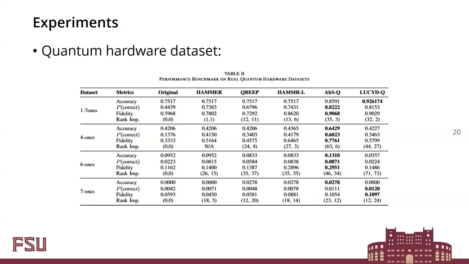
In simulation under a scaled noise model of an IBM machine, Tran reported a clear lead, an accuracy of 0.82 at a noise level where rival methods sat at or near zero. Hardware results were weaker. An older network, AbS-Q, kept a slightly higher probability and fidelity on a mixed set of targets and led on two harder sets, and Tran called some of the hardware figures too small to count as a result.

Checking before voting lifts precision from 0.22 to 0.95

Kausthubh Chandramouli of North Carolina State University presented work with Mohsen Ghodrati and Dror Baron. It targets algorithms whose answer is a bit string, such as Grover search. Majority voting on each bit can rebuild a string that never turned up among the shots. In their example it took 23 shots on 500 qubits at a 5 percent flip rate, where waiting to see the true string would take more than 10 to the 11.

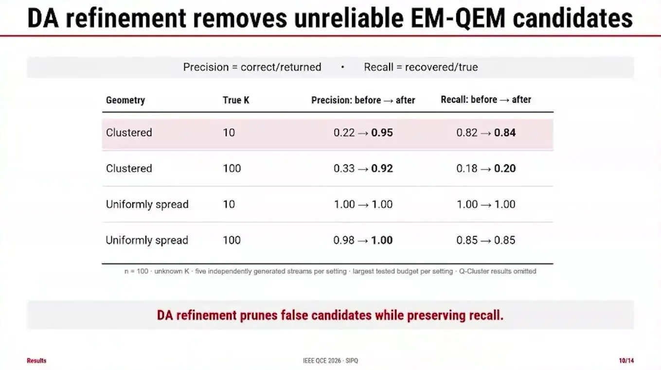
With several right answers, voting must run within regions of the data, and tools called Q-Cluster and EM-QEM form those regions. Chandramouli calls a region dominated when each bit’s vote favours the true answer by more than half, which restores the voting guarantee. Checking for that before accepting a result raised EM-QEM’s precision from 0.22 to 0.95 on clustered test data with ten true answers, while recall held. The noise model is kept simple on purpose. Detailed models, Chandramouli said, stop the fit from settling.

Faster readout repaired in software

Jadwiga Wilkens, a PhD student at Johannes Kepler University Linz, presented work with Alpine Quantum Technologies, or AQT. The firm reads each trapped ion with a pulse of light that lasts 1.5 milliseconds. The team asked whether a shorter, noisier pulse could be fixed in software, using a method called robust shadows that first measures how each qubit’s readout goes wrong and then corrects for it. Mostly it could, the team reported.

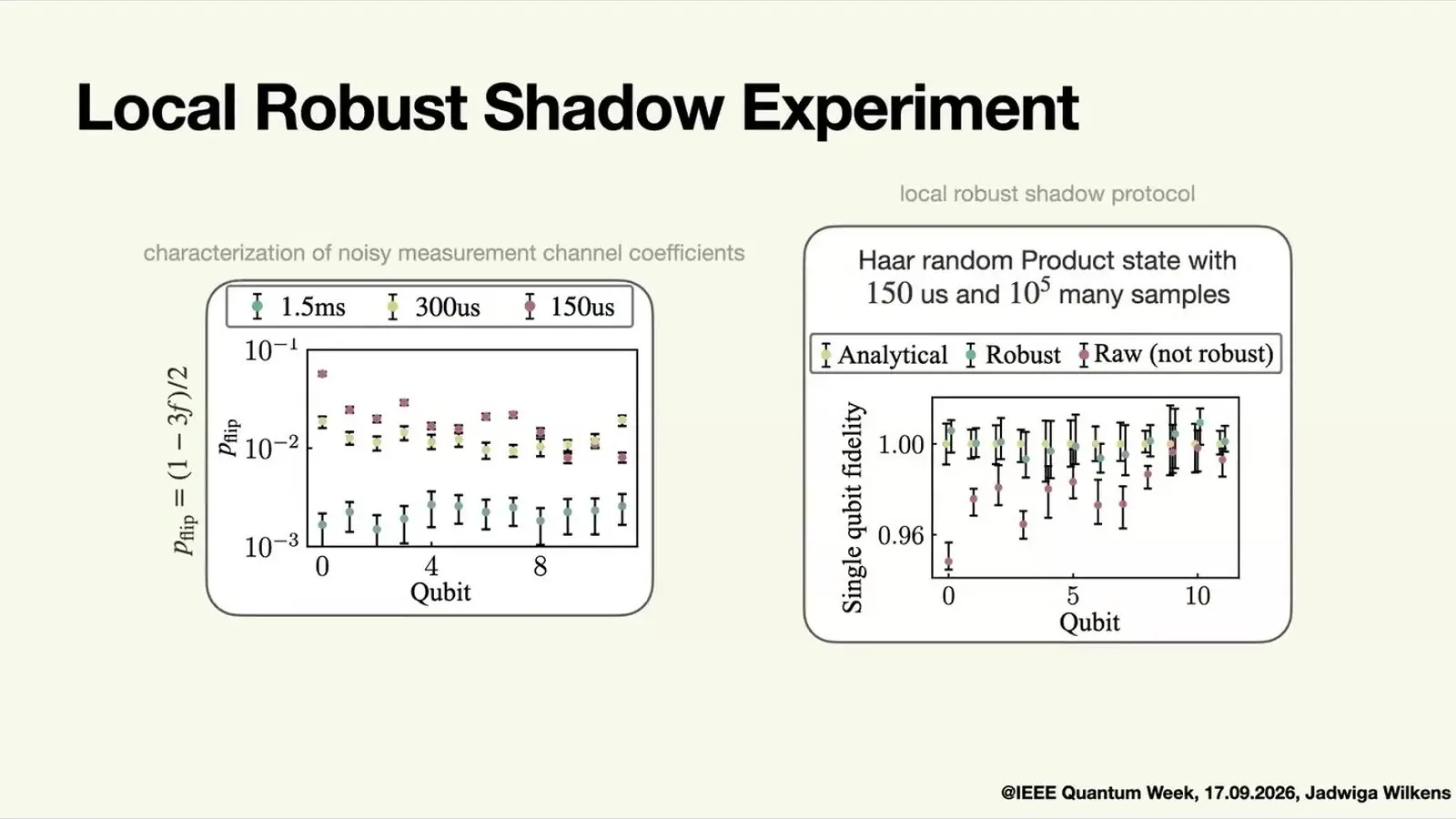
The test machine had 12 calcium ions. The pulse was cut to 300 and then 150 microseconds, and at 150 the raw single-qubit scores dipped to about 0.95 while the fixed estimates came back to the expected value. A nine-qubit circuit gained only a little. Wilkens traced that to noisy two-qubit gates, and the team said a tenfold shorter readout trims total run time by at most 5 percent on AQT’s set-up.

A genetic search for better pulse shields

Kevin Joven Noriega, a quantum benchmarking intern at QED-C, tackled dynamic circuits, which measure qubits partway through and use the result to choose later gates. Waiting qubits lose their state while the controller works. Short runs of pulses that add up to nothing can shield them.

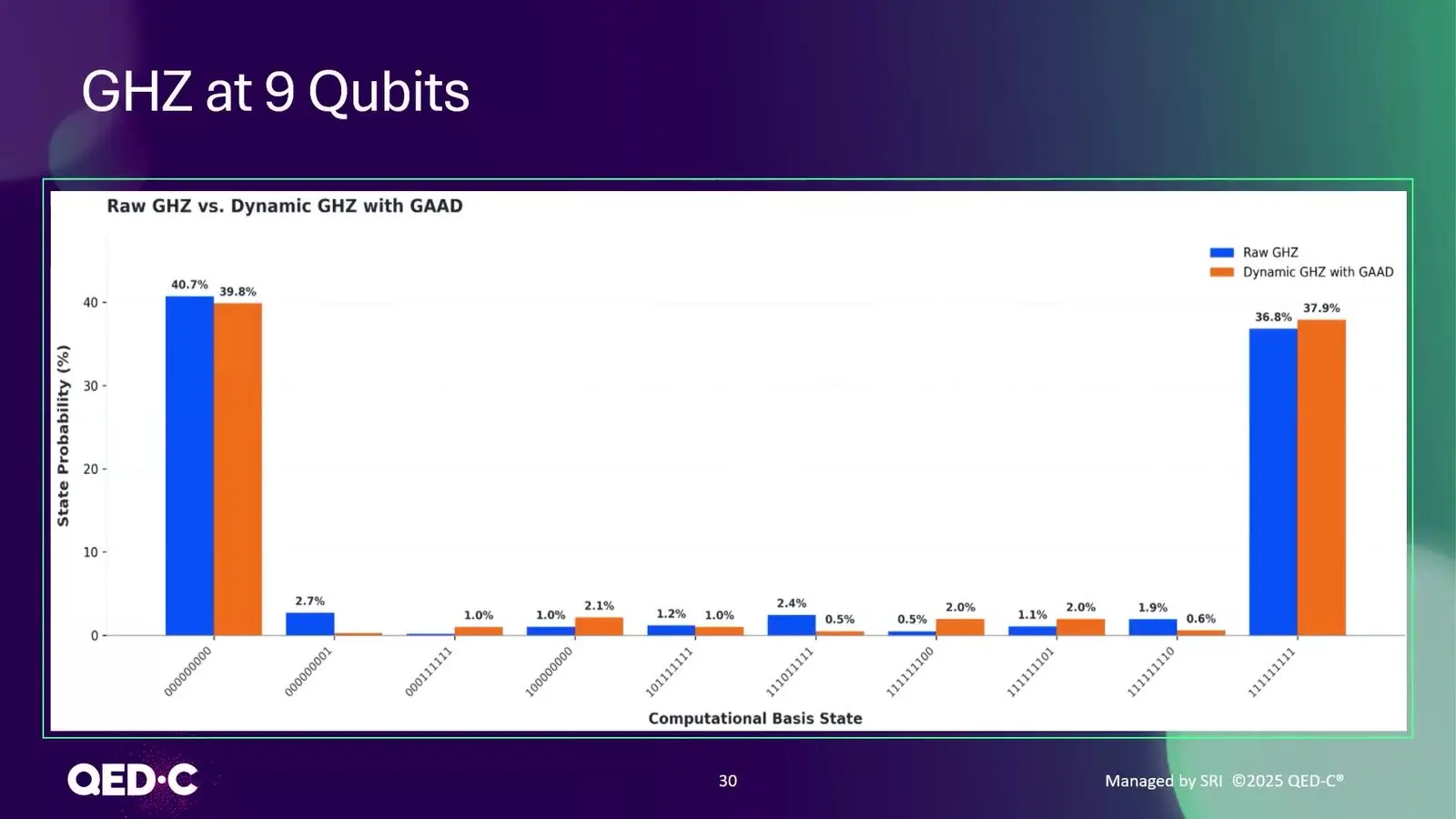
Joven Noriega used a genetic algorithm to breed better pulse runs on hardware. On a nine-qubit test state on IBM hardware, the tuned circuit put 77.7 percent of shots in the right two outcomes, against 77.5 percent for the plain circuit. Noriega said the team aims to repeat the test at 50 to 70 qubits.

Error detection lifts a graph state 235-fold on IBM hardware

Ali Javadi-Abhari, who leads Qiskit at IBM Research, gave the Tuesday keynote. Javadi-Abhari puts all three ways of dealing with errors on one trade-off, with time counted in samples and space in qubits. Mitigation takes many blurry pictures. Correction builds the spare copies into the camera. In the long run full fault tolerance wins, Javadi-Abhari said, but for now the fixed costs of each method decide what can be done on the machines that exist.

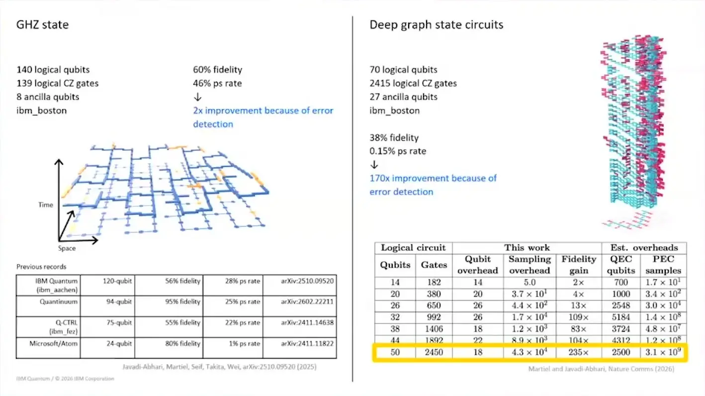
On ibm_boston, error detection lifted the fidelity of a 50-qubit graph state 235 times. It took 18 extra qubits and 43,000 times the usual number of samples. The rivals cost far more, since full surface-code correction would need an estimated 2,500 qubits and error cancellation on its own 3.1 billion samples. The two tools also mix. In a 20-site Ising model laid onto 49 qubits, adding detection to cancellation cut the bill in samples 88 times.

The keynote also held a warning for the auditors. On a 56-qubit echo test, two leading classical methods disagreed with each other, while mitigated results from different IBM chips agreed. At the far end of the path, a stacked gross code reached a logical error near 4 in 10 to the 15 in simulation. Javadi-Abhari conceded that decoding such dense codes in real time is still hard.

Symmetry checks cut error cancellation’s shot bill 16-fold

Caleb Johnson, a software engineer at IBM Quantum, taught a two-part tutorial on the Tuesday on probabilistic error cancellation in Qiskit. The method learns each layer’s noise. It then runs many random circuits whose signed average undoes that noise, and Johnson stressed that it is free of bias only when the noise model is right and enough samples are taken. Shaded light cones, which drop tiny noise terms inside the measured value’s light cone, were what made a 56-qubit echo of about 1,000 two-qubit gates feasible, Johnson said.

The second session ran the notebooks on 49 qubits of IBM Boston. The test was a 22-site Ising model on IBM’s heavy-hex chip, where 27 go-between qubits should end in the ground state, so any that reads 1 marks a shot to throw away. Every noise term those checks can catch was struck from the model. The shot multiplier fell from 100 to about 6.25, roughly the gap between six hours and half an hour on the machine.

A state-vector simulator gives exact values for this model, so every step of the demonstration could be checked against the truth. Johnson made no claim of advantage. About 30 percent of shots survived the checks.

How a value is measured decides whether backpropagation pays

Kevin Dougherty, a pre-doctoral researcher at Argonne, presented a paper with Ji Liu. Operator backpropagation pushes the measured value back through part of a deep circuit on a classical computer, so a shorter circuit is left for the quantum machine. The catch is cost. The number of terms to measure grows fast, so Dougherty tried two ways to measure them, commuting groups and derandomised shadows, whose shot count grows only with the log of the number of terms.

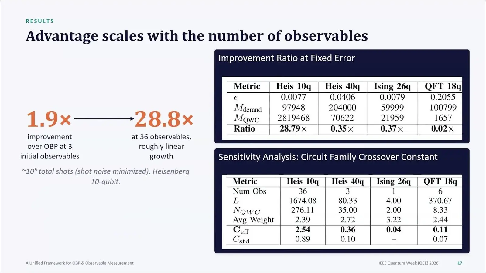
On a Heisenberg circuit, backpropagation cut the depth from 90 to 10. At about 100,000 shots on a 10-qubit case, the saving from shadows rose from 1.9 times at three observables to 28.8 times at 36. Other circuits went the other way. On three of them the ratio fell below one, as low as 0.02, which Dougherty read as the commuting groups winning.

Learning what the hardware really does

A single score hides how a machine goes wrong. Ten talks sought richer models of real machines, often from data that users produce anyway, and one built a simulator that copies the whole machine, controller and all.

A cheap probe for drift on cloud machines

Yi-Ting (Tim) Chen of Amazon Braket presented work with Aniket Dalvi and Nils Quetschlich. Their subject was drift, the slow change in a machine between calibrations. On a cloud service every minute spent checking a machine is a minute taken from customers, so the team wanted the most information for the least machine time.

The plan has two tiers. A light probe runs often, and full benchmarking runs only when the probe raises an alarm. At an equal cost of 68 circuits, the probe caught drift 73 percent of the time against 5 percent for tuned benchmarking at one drift level. Chen named their simple decay model as the main limit.

Learning how analogue machines respond

Andrey Lokhov of Los Alamos National Laboratory presented work with Cenk Tüysüz, Abhijith Jayakumar, Carleton Coffrin and Marc Vuffray. Analogue machines take an energy rule as input. The team maps what the user asked for to what the machine did, and it learns that map from normal user jobs so that nobody has to book the machine.

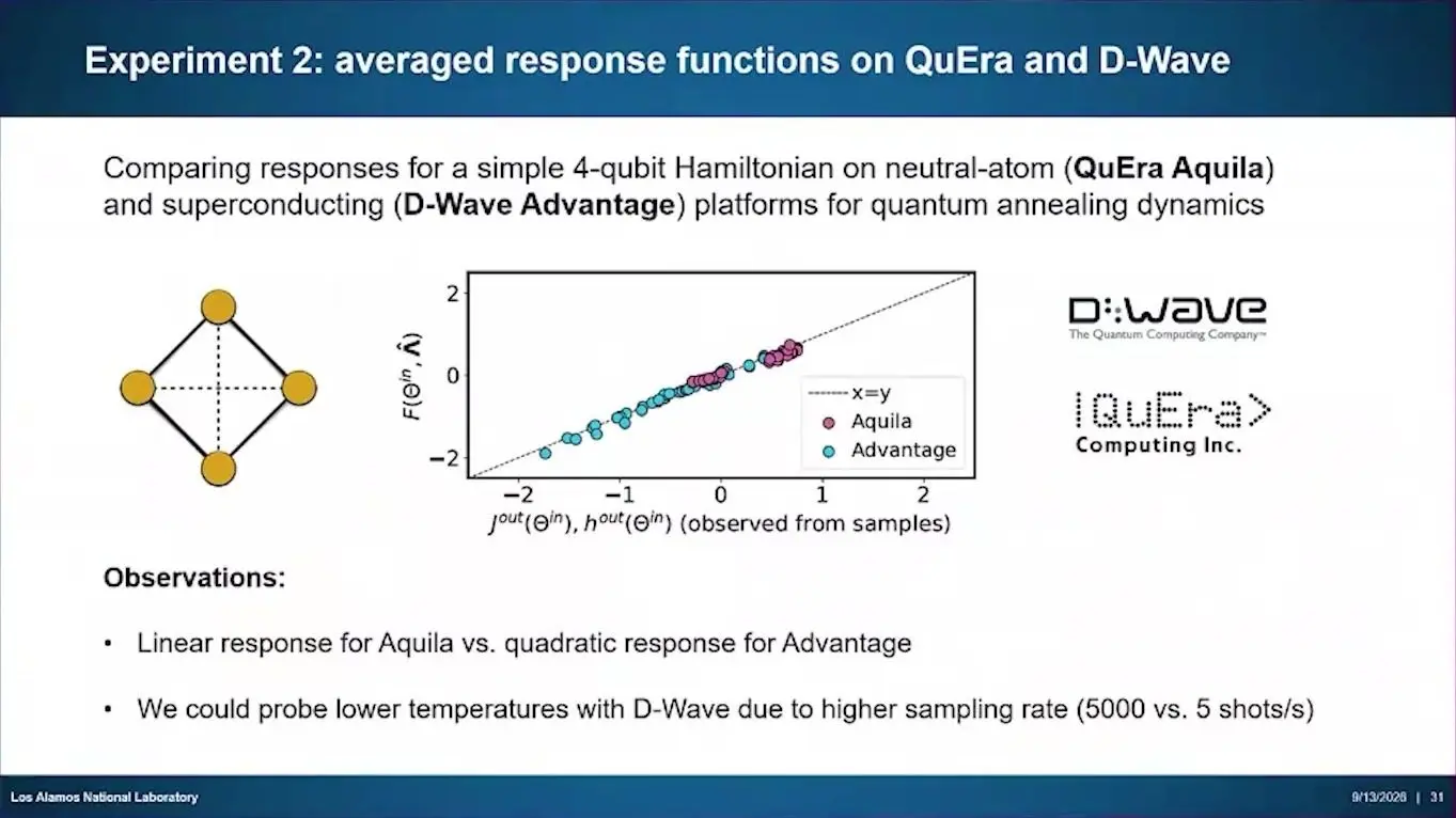
A four-qubit test found a simple, straight-line response on QuEra’s Aquila and a curved one on D-Wave’s Advantage. Lokhov traced the curve to stray links between qubits that are not wired together at all, which the newer D-Wave chip showed less of than the older one. QuEra’s machine could only be probed lightly. It takes about 5 shots a second, against 5,000 for D-Wave’s.

Checking each branch of a teleportation

Mason Edwards of the University of Florida presented work with Prabhat Mishra. In teleportation one side measures two qubits and the other applies one of four fixes, chosen by what the first side saw. Most tests report only the average across those four branches, Edwards said. Their method checks each one.

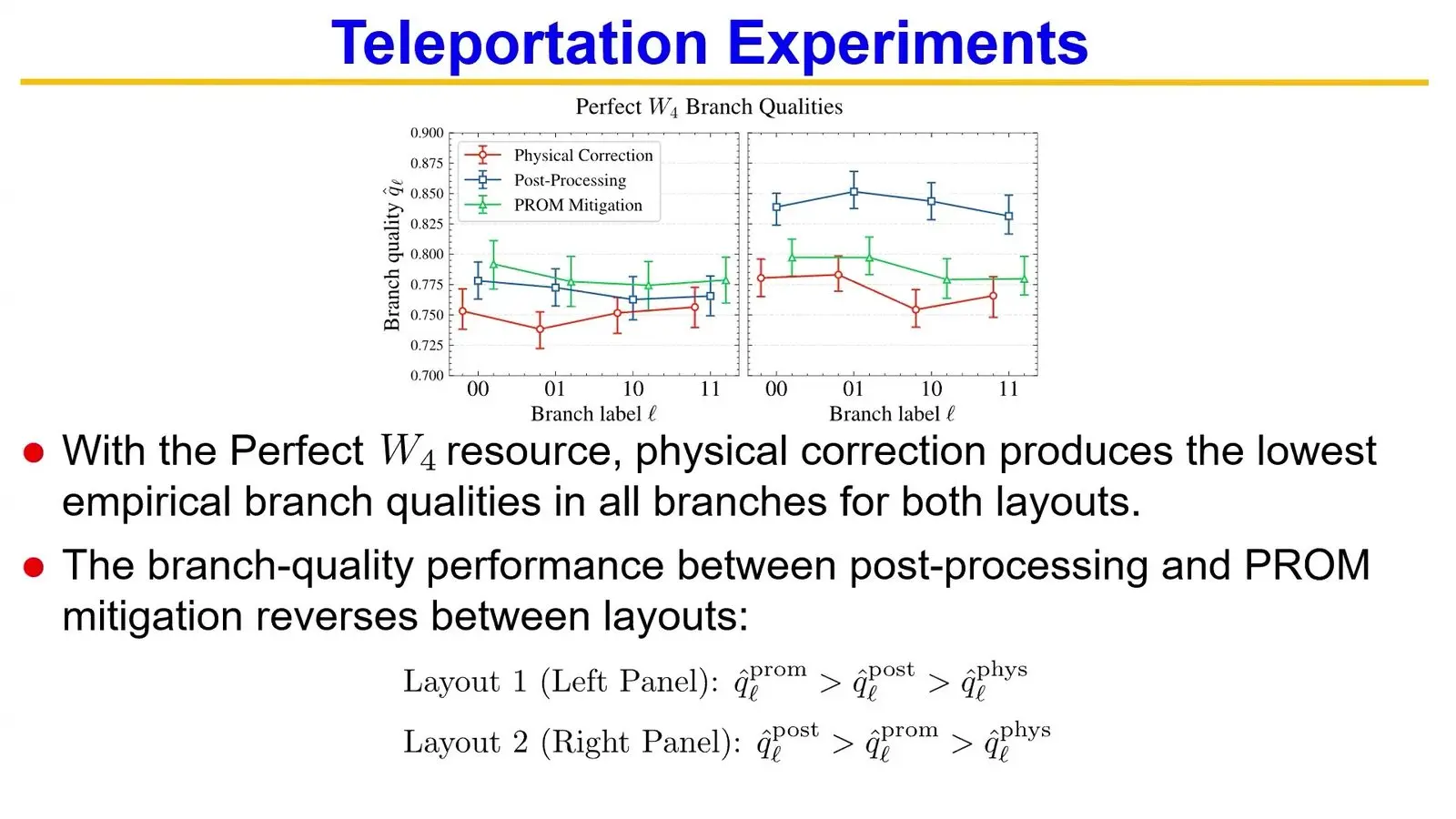
All runs used IBM’s 156-qubit Fez processor. Applying the fix live, from a measurement in the middle of the circuit, was worst in every branch. The order of the other two methods flipped between qubit layouts, and Edwards tied that to the chance of a misread outcome, about 6.9 percent on one layout against 1.2 percent on the other.

A noise model trained on one run

Ryo Sakai of JIJ presented work with Yu Yamashiro. Vendor figures for single gates do not add up to a model of the whole device, Sakai said, while full testing is costly and covers one gate at a time. Sakai wanted a noise model trained on one ordinary run that carries over to other circuits.

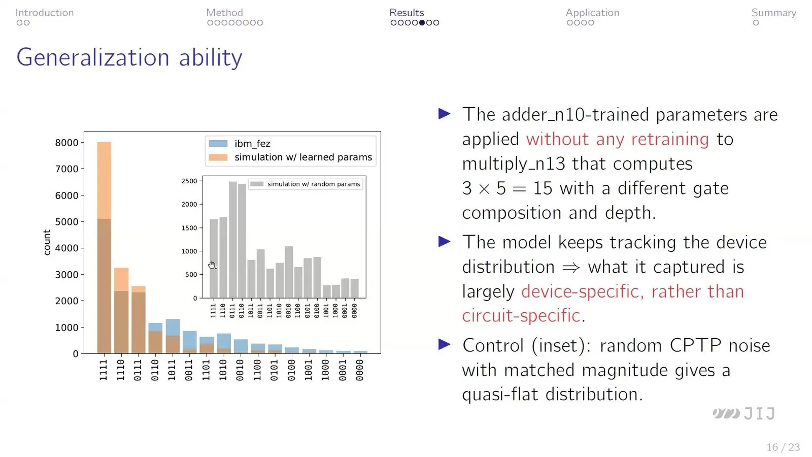
Training used one run of a 10-qubit adder on IBM’s Fez. It had 16,384 shots. Applied unchanged to a multiplier circuit, the model still tracked the device, and the learned two-qubit gate error came out at 2.03 percent against IBM’s median of about 0.25 percent. Sakai called their numbers an effective error budget and put the gap down to deliberate simplification in the model.

Google learns the true rules of its analogue chip

Nikita Astrakhantsev of Google Quantum AI runs Google’s chip in analogue mode, with all its couplers on so the qubits evolve under one fixed energy rule. Nobody knows exactly which rule the chip applies. In the group’s 2024 work, Astrakhantsev said, about three times more error came from using the wrong model than from qubits losing their state.

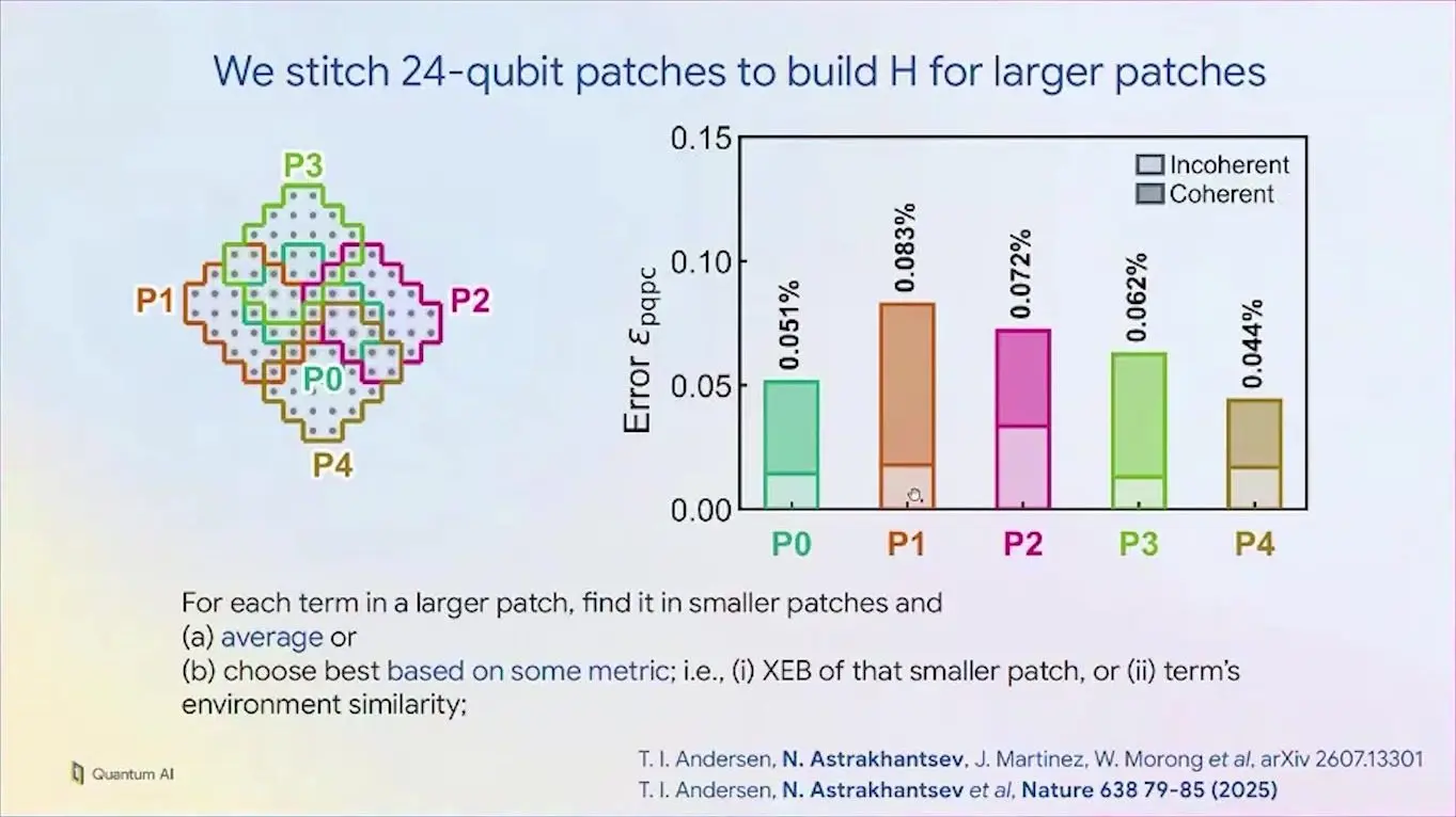
Their team tunes a model with about 40 settings per qubit until its predictions match the samples. One step on 30 qubits takes six hours, so they train 24-qubit patches. From a poor starting point Astrakhantsev reported errors cut by up to 50 times, which let the team study how waves of flipped spins fade on the chip.

A simulator that copies the whole machine

Xiu-Zhe (Roger) Luo of QuEra argued that simulation should copy what a real machine does, from its classical controller and the optics that move atoms to the quantum circuit and the decoder. Luo’s answer, PPVM, is written in Rust and runs one program that mixes classical steps, quantum gates and noise such as lost atoms.

Luo ran it live in a browser. Luo took about 1,000 noisy shots of a fault-tolerant protocol and watched the decoding graph grow on screen. AI agents tuned its speed for days against a set of tests, and one change they kept cut a workload from 2.62 to 0.52 seconds.

A tensor-network twin of 64 Rydberg atoms

Simone Montangero of the University of Padua argued that a classical twin of a chip should model its energy rule, its control pulses and its compiler together, up to hundreds of qubits. Then the effects among many qubits that a gate model misses come into view. But a twin good enough to replace the machine would make the machine pointless. So a useful twin, Montangero said, stops short.

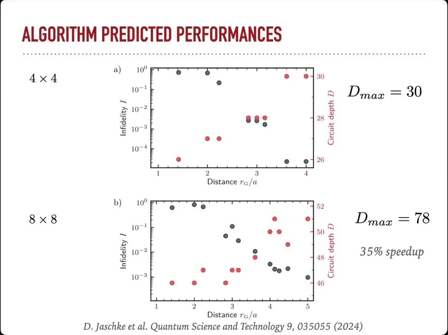
The worked example made a GHZ state, in which all qubits are 0 together or 1 together, on 64 Rydberg atoms in an 8 by 8 grid. The device numbers came from a Stuttgart test. On that grid the twin needed a bond dimension, its gauge of how much entanglement it keeps, of 78, and its plot marked a 35 percent speed-up. Montangero warned that multiplying two-qubit errors together does not give the error of the whole state.

Vendors’ noise data is the missing piece for twins

A panel chaired by Antonio Andrea Gentile of Pasqal closed the Quantum Engineering Cycle workshop on the Tuesday. It named one main barrier to faithful twins. Vendors do not share enough noise data. Yuri Alexeev of NVIDIA said they hold back detailed tomography for fear that rivals will copy their designs, and proposed a shared store of such data in one standard format.

Montangero thought the tools already exist. The rule of thumb Montangero gave was to switch to tensor networks beyond 40 to 45 qubits for closed systems, or 12 to 15 for open ones. Aleksander Wennersteen said Pasqal writes many small emulators for set tasks in place of one big one, and Andrea Delgado of Qblox named integration as the place where time will be tight.

Shadow fingerprints tell ten noise types apart

Lei Zhang of UMBC presented work led by Vridhi Jain, now at the University of Delaware. The aim was to name the kind of noise on a machine without full process tomography, which is costly. Nine small probe circuits ran under ten noise models from Qiskit Aer, among them bit flip, amplitude damping and reset, and each probe was measured on random axes, a method called classical shadows.

Three kinds of classifier all landed near 70 percent accuracy on 10,000 simulated fingerprints. Reset noise was often mistaken for amplitude damping. Both push qubits toward zero. Asked how stable a fingerprint would be on real machines, Zhang called that an open problem, since real noise drifts more than simulated noise does.

Fifteen circuits confirm a 42-qubit GHZ state

Vincent Russo presented a paper with Farrokh Labib, David Nicholaeff and William Zeng. A GHZ state is a common hardware test, and part of its fidelity shows up as a wave when every qubit is turned by the same angle. Sampling that wave evenly takes about 2N circuits for N qubits. Because the wave has one known frequency, Russo samples random angles and uses the Lasso, a fit that drives weak candidates to zero, to find it.

In simulation, about 15 angles were enough at 42 qubits. For trapped-ion machines, whose qubits all link to each other, a GHZ circuit can be built as a shallow tree, and checks between pairs of its end qubits catch faults along the way. The method ships in the open-source metriq-gym package. A 26-qubit run on a Quantinuum emulator gave a coherence of 0.906.

Quantum benchmarking choices that change the ranking

Seven talks showed how much a headline result depends on what is counted. Classical filtering, the choice of classical rival, queue time, price and the cost of simulation all moved the answer.

How much of a D-Wave result is classical filtering

A University of Toronto team tested graph matching on D-Wave’s Advantage2 annealer. The authors are Akhtar, Wrona, Chowdhury and Mahmoud. They asked how much of a good run belongs to the classical filter that runs before the annealer ever sees the problem. The filter turned out to do much of the work. At 50 vertices a strong filter left the annealer nothing to do at all in 5 of the 16 set-ups the team tried.

A standard classical routine solved every normal case in under 10 milliseconds. The team claimed no quantum advantage, and it said so plainly in the talk.

A quantum reservoir against a tuned classical twin

Tushar Pandey, who works at DataRobot and spoke on their own research, reran quantum reservoir computing against classical models given the same tuning budget. In a reservoir model a fixed quantum system holds the signal and only a simple readout is trained, which makes it cheap to try on today’s machines. It did well at first. The quantum reservoir beat a default classical network on a standard chaotic test, then lost, 0.73 error against 0.36, to a classical model of matched size.

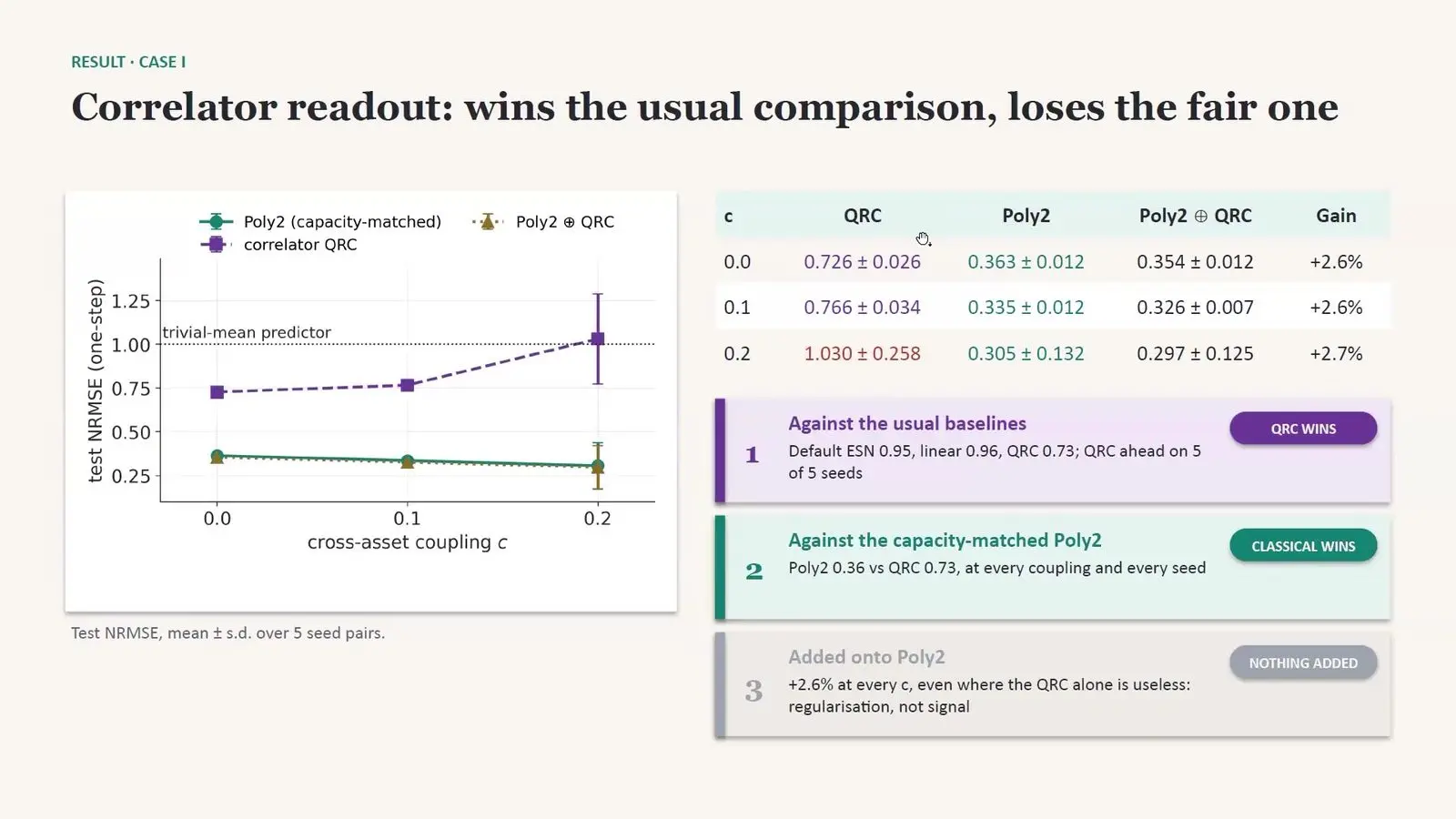
Adding the quantum features to the classical model gained 2.6 percent, which Pandey read as a smoothing effect that brought no new signal. Pandey argued that any claim of quantum gain should name a tuned classical twin.

Price reorders the leaderboard

Siddarth Shinde of Northwestern University presented work with Jakub Szefer on a new score. It divides how close a machine’s output comes to the ideal by what the run cost, so a score of 608, Shinde said, means 608 usable shots for each dollar spent. Price now sits beside quality.

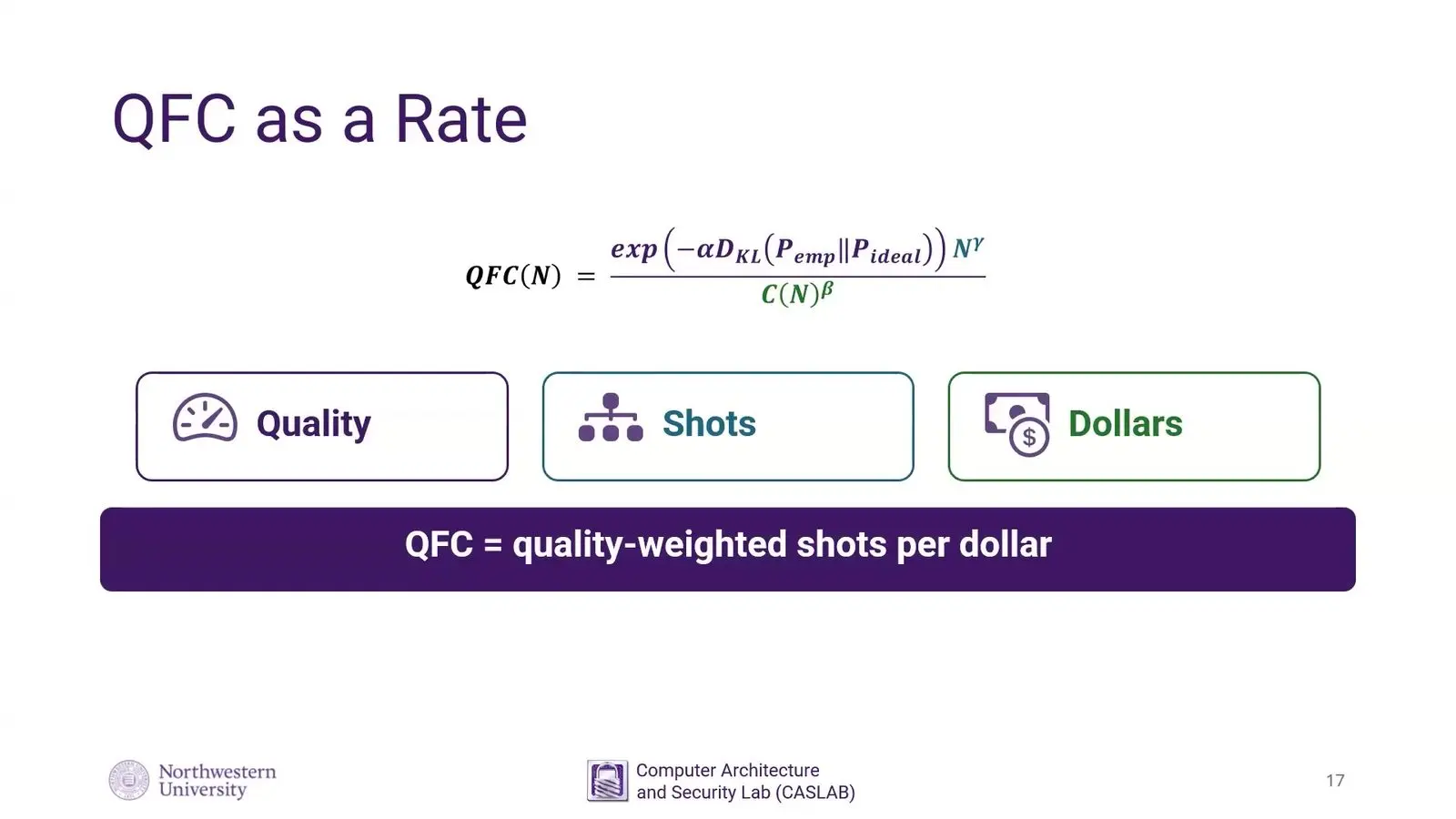
The team logged 247 runs on 12 processors through 14 access routes across four clouds. On fidelity alone IonQ’s Aria led and IQM’s Sirius sat ninth, while on the priced score Sirius led at about 47 times the bottom entry. Seven IBM machines under one billing model spanned a factor of 17. The test circuit was a simple two-qubit state.

Ember tests how problems fit onto annealers

Unmol Sharma, Zachary Macaskill-Smith and Melissa Warner of Vanderbilt University presented Ember, a test suite for how a problem is laid onto an annealer’s chip. The chip is sparsely wired. So each variable in a problem is spread over a chain of qubits, and long chains break more often and waste qubits.

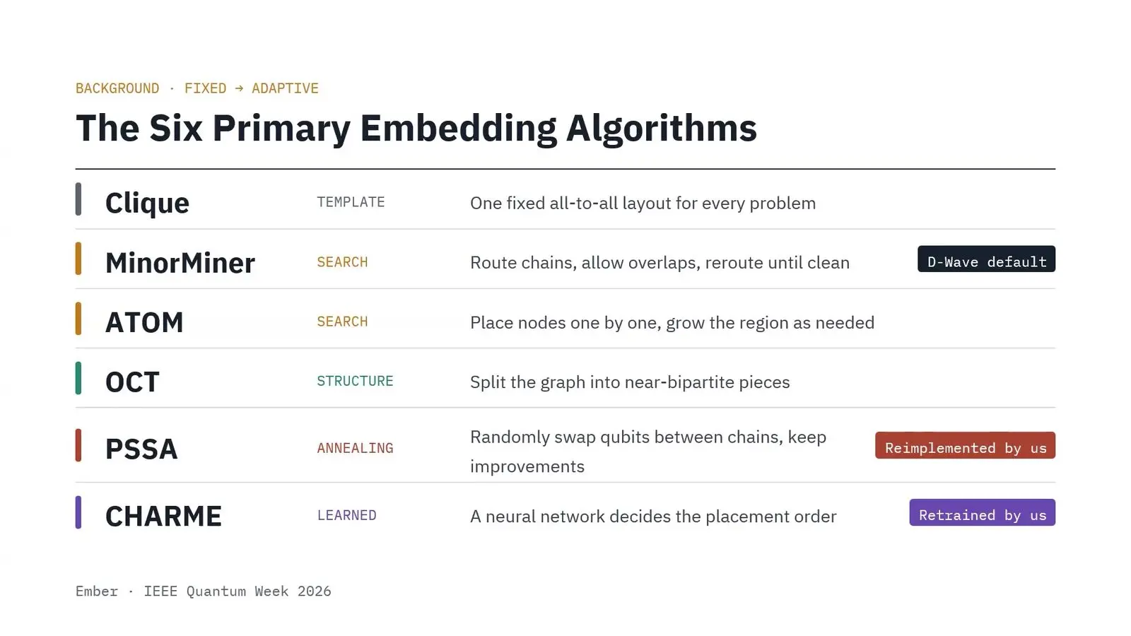
The suite holds about 24,000 graphs and compares six methods. MinorMiner, D-Wave’s default, led by about 20 percent on success and made shorter chains, and a neural method lost to it even after the team retrained it on its own graphs. No annealer ran in the loop. So the scores measure the fit alone and leave out the answers a user would read.

Qubit count alone does not set the cost of simulation

Haoyuan Tian, a doctoral student at William and Mary, presented work with their advisor Jie Ren. The question was where the time goes. Tian split the cost of simulating a circuit into three jobs, evolving the state, drawing samples and checking the result, and timed each one for three simulation methods. On 16 qubits, one method on an ordinary processor slowed more than 5,200-fold as a random step run before the main circuit got deeper. The same chain method on a graphics card slowed sixfold, and the full-state and tensor-network methods barely moved.

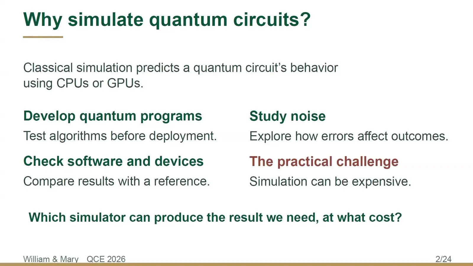
Tian’s point was that qubit count alone does not set the cost. Tian advised moving off the full-state method beyond about 32 qubits on one A100 card, and reporting the quality of any shortcut beside its cost.

Counting queue time erases a QAOA training edge

Davide Venturelli of USRA’s Research Institute for Advanced Computer Science wants every quantum heuristic sold with a window sticker. That is a plot of how good the answer is against the time and resources spent, as already drawn for a coherent Ising machine set against simulated annealing. Optimisation suits it. The answer is a bit string, and anyone can check how good it is.

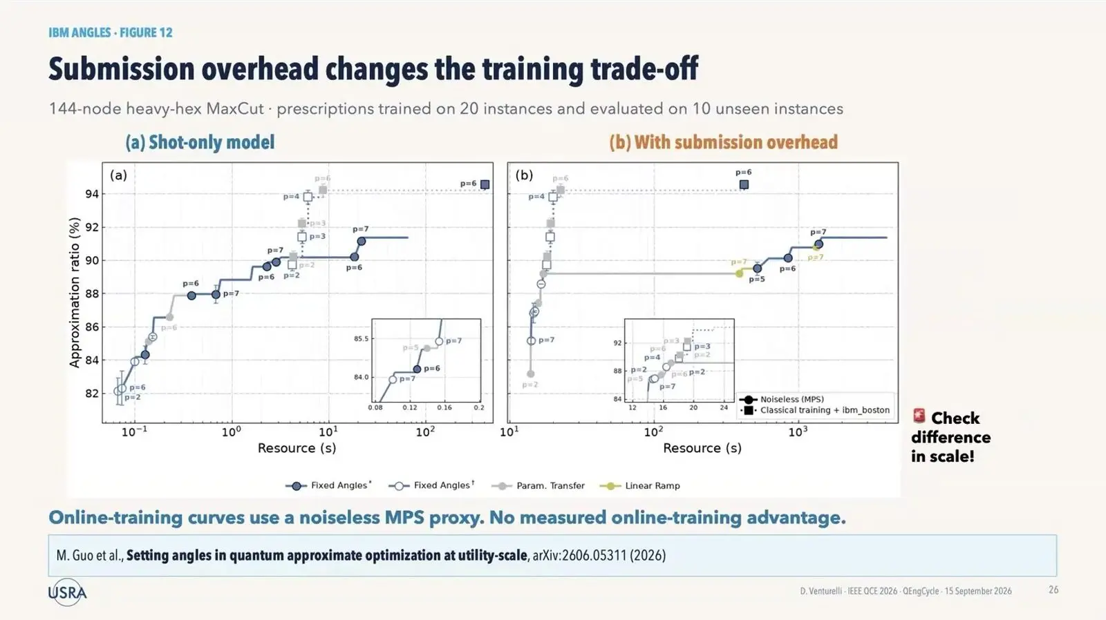
In a study with IBM on 144-node MaxCut on ibm_boston, training QAOA on the hardware looked like a gain. Then the time to submit jobs was counted. No measured edge was left. Venturelli put quantum optimisation about three orders of magnitude behind on speed, problem size and the handling of constraints, and expected many end-to-end benchmarks within two years.

A stronger classical rival shrinks a sampler’s lead ninefold

Arul Mazumder of Carnegie Mellon University tested an ideal quantum sampler on Markov random fields. These are graph models whose classical samplers mix slowly when the graph has loops. The yardstick was effective sample size, the number of truly separate samples a run is worth, and across 60 cases in five families of graph the quantum sampler beat plain Gibbs sampling by 16.35 times. Then the rival changed. Against parallel tempering, a stronger classical method, the lead fell to 1.79 times.

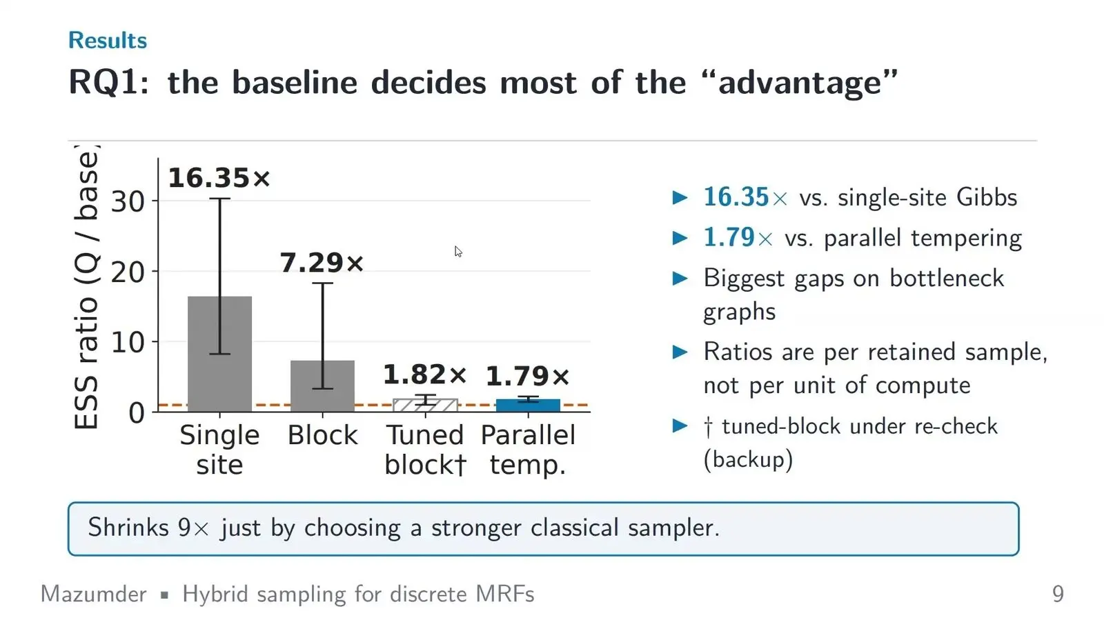
On wall-clock time there was no gain at all. From the same full table of odds, exact classical sampling on a CPU ran 1.34 times faster than the simulated quantum sampler. Shallow circuits also lost to simple classical guesses on these sharply peaked targets, and Mazumder put that down to the limited depth of the circuits.

Standards bodies try to make the numbers comparable

If auditors are to check vendors, everyone needs shared yardsticks. Three talks set out where the standards work stands, one on the Wednesday and two on the Thursday.

Benchmarks must cover the whole hybrid workflow

Tadashi Kadowaki of AIST argued on the Wednesday that a test of the quantum step alone misses most of the cost. Take a protein-ligand study run on two IBM machines with Fugaku and another supercomputer, which used more than 150,000 Fugaku nodes at peak and was a finalist for the ACM Gordon Bell Prize this year. Future systems will mix CPUs, GPUs and quantum chips. So Kadowaki asks how well the whole system solves a useful problem.

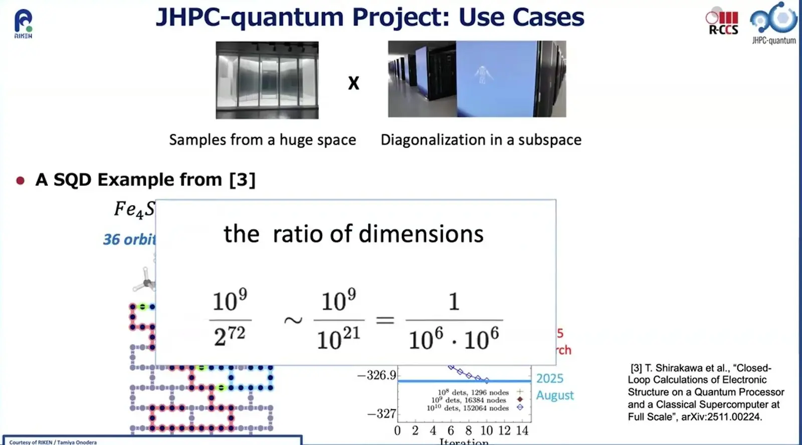
A RIKEN-led project, JHPC-quantum, links quantum computers to big supercomputers, and its test user scheme took 21 proposals this year. Japan is also drafting a technical specification for the middleware layer of hybrid benchmarks under IEC and ISO JTC 3. It is not yet an approved project. Nor will it set out a list of tests.

ISO and IEC sort the benchmarks

Masahiro Horibe, deputy director of AIST’s G-QuAT centre in Japan, leads the benchmark group of the joint IEC and ISO quantum committee. Nearly everyone agrees these standards matter, Horibe said. But each pictures them in a different way, so the group first wants a shared frame that sorts tests into several kinds, from use-case and algorithm benchmarks down to processor benchmarks.

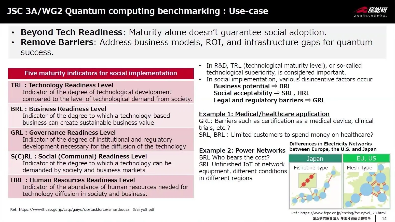
Horibe also described ABCI-Q, AIST’s platform of 2,020 NVIDIA H100 cards joined to quantum machines from Fujitsu, QuEra and OptQC. Horibe was blunt about vendors. Asked about one benchmark promoted at the meeting that week, Horibe said every vendor tells users on tight budgets it is number one. Better tests would match a type of machine to an industry.

QED-C tracks error-correction claims

Bruno Avritzer of Leidos, vice chair of QED-C’s standards committee, said company webinars this year showed no agreement on what quantum advantage means. QED-C keeps an open test suite. It has more than 16 programs and runs on hardware from IBM, IonQ, Quantinuum, Rigetti and IQM, and the group now plans a shared tracker of error-correction results with their circuits and fidelities.

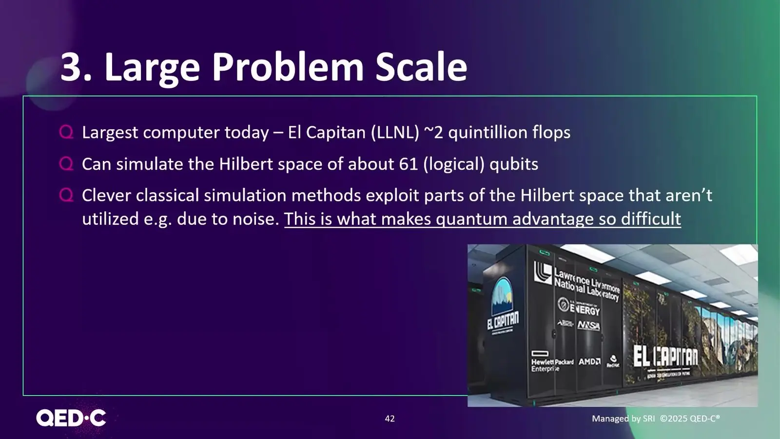
The floor pushed back. One questioner said the week’s benchmarks would not pass in a policy discussion because outsiders cannot verify them. Avritzer agreed vendors will not hand over machines for retesting, so the aim is full disclosure of what was run.

Open benchmark suites and shared data

Shared yardsticks need shared tools. Six talks in the Wednesday QuBench workshop offered new scores, open suites and a public store of results.

QUOPS ranks Helios-1 well ahead of Willow and Boston

Oliver Widzowski Maupin of Sandia National Laboratories presented QUOPS, a score built with Quantinuum and NVIDIA. It gives the size of the largest circuit a machine runs well, and how many such operations it gets through each second. The test circuits are random layers of gates. Each one is checked with a mirror circuit, which runs a circuit and then its reverse, so that the right answer at the end is known in advance.

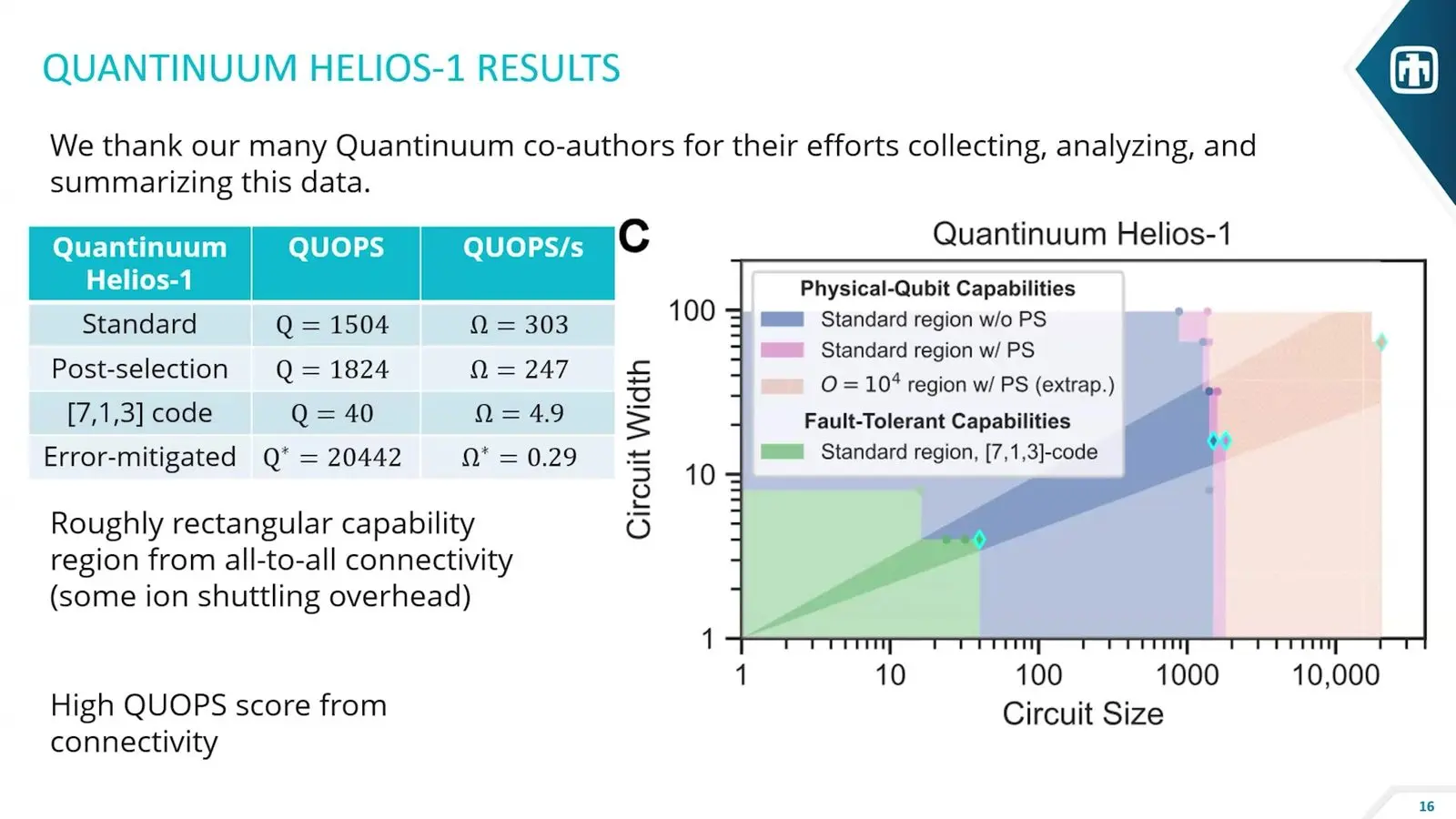
Quantinuum’s Helios-1 scored 1504 at 303 operations per second, against 216 each for Google’s Willow and IBM’s Boston. With logical qubits in the Steane code, Helios-1 scored 40. Widzowski Maupin called the day a logical machine beats a physical one on QUOPS a milestone, and put useful work at roughly 10 to the 8.

Blind tests certify a device without noise assumptions

Elham Kashefi of the University of Edinburgh, chief scientist at the UK National Quantum Computing Centre, said error correction, error mitigation and most benchmarks all make a guess about the noise. No vendor offers a check on a device’s output that is free of such guesses. So Kashefi’s group hides test runs among real runs, using blind computing built on measurement. The device cannot tell which is which, and the method has run on Quantinuum’s H1.

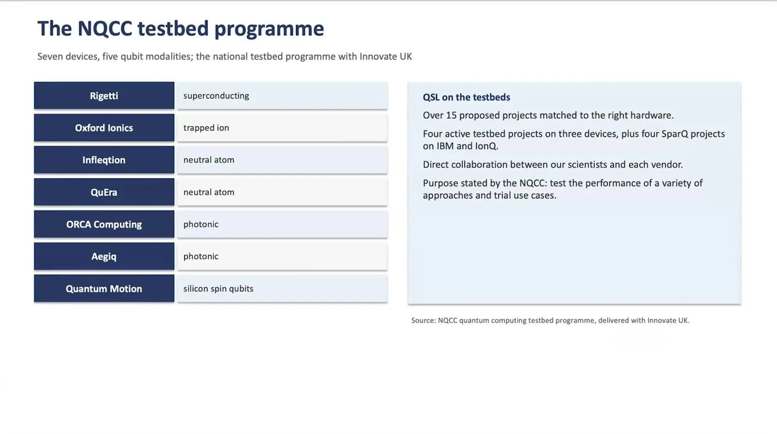
The main lesson from the centre’s seven test machines was that each experiment still needs its own tailored benchmark. A new programme, Quantum Advantage TurboCharger, has 20 million pounds to spend from 2026 to 2030, and its core is checking results. Kashefi proposed a certified QUOPS.

One file format for optimisation benchmarks

Yu Yamashiro, chief executive of JIJ in Tokyo, argued that an optimisation benchmark turns on far more than the solver. How a problem is written, changes to the data, classical steps and the rules for scoring all shift the result. JijModeling writes a model once. OMMX then stores problems, answers and records in one form that moves between tools, with links to classical solvers, annealers and gate-based services.

OMMX can read QOBLIB, a library of hard problem types. A benchmark run, in Yamashiro’s account, should record the score of the answer, whether it obeys the rules, the gap to the best known answer and which steps before and after the solver were counted. Yamashiro is also a co-author of the noise-model paper Ryo Sakai presented.

MQT Bench keeps loops as loops

Damian Rovara of the Technical University of Munich, speaking for Robert Wille, argued that unrolling loops before compiling wastes effort. An unrolled eight-step Grover circuit sprawls. Its looped form stays fixed in size. MQT Bench makes test circuits at four levels, from the bare algorithm down to a version mapped onto one chip’s wiring.

New in the suite are dynamic circuits, which measure qubits partway through, and loops written straight in OpenQASM. Rovara reported more than 400 citations and more than 160,000 downloads. The suite has spread. Rovara also suggested the Jeff exchange format, backed by compiler teams at Xanadu and Quantinuum, could carry such tests from one tool to the next.

Most benchmarks measure one noise budget

Alessandro Cosentino of the Unitary Foundation opened Metriq-data, a public store of hardware results. Each result is a checked record in a public Git store, with the device version, the time of its last tune-up, the software used and the settings all attached. By 15 September 2026 it held more than 400 results. They came from 18 devices.

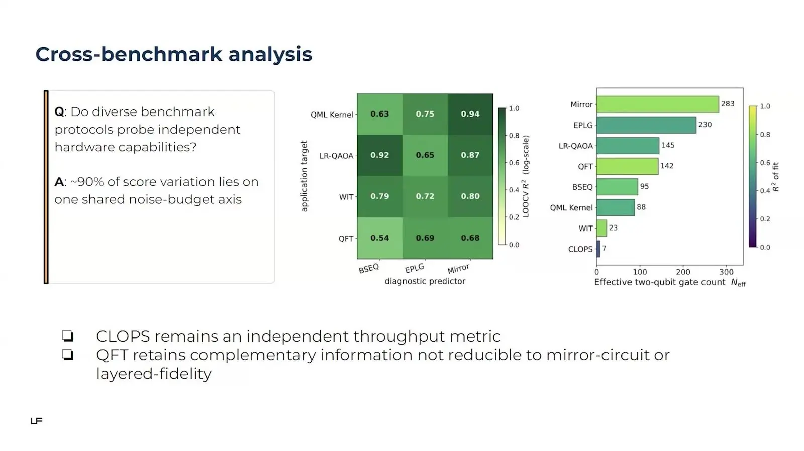
About 90 percent of the spread in scores lay on one shared noise axis, Cosentino reported. That is close to what two-qubit gate error alone would predict. CLOPS, IBM’s speed measure, and a Fourier-transform test carried facts the others did not, and most of the project’s effort, Cosentino said, goes into running the same circuits through different cloud front ends.

Five years for quantum volume to catch on

Valentin Gilbert of the Quantum Benchmarking Zoo, a volunteer-run French project, judges a metric by whether others use it. Gilbert scores a point each time someone else adopts a protocol. Other hardware makers took about five years to start reporting quantum volume after IBM introduced it in 2017, and IBM itself dropped it for error per layered gate in 2023.

Fidelity is the figure most often reported, Gilbert said, yet the fidelities that come from different tests cannot be set side by side. Add Cosentino’s finding that eight benchmarks largely track one noise budget, and the field seems to make up scores faster than it uses them.

Faster classical simulators for checking and design

The audit needs tools. Eight talks set out faster ways to simulate circuits on ordinary hardware, half in the Tuesday simulation workshop and the rest in Wednesday paper sessions.

A contraction schedule that spots easy problems

Stefanos Kourtis of the Université de Sherbrooke and Institut Quantique started from a puzzle in the group’s own work. Tensor networks had cut the cost of Google’s 2019 Sycamore circuits from an estimated 10,000 years to hours on graphics cards. Yet they choked on sums that are easy. On linear equations modulo 2, which Gaussian elimination solves at once, the cost of the network turned exponential past a certain density of rules.

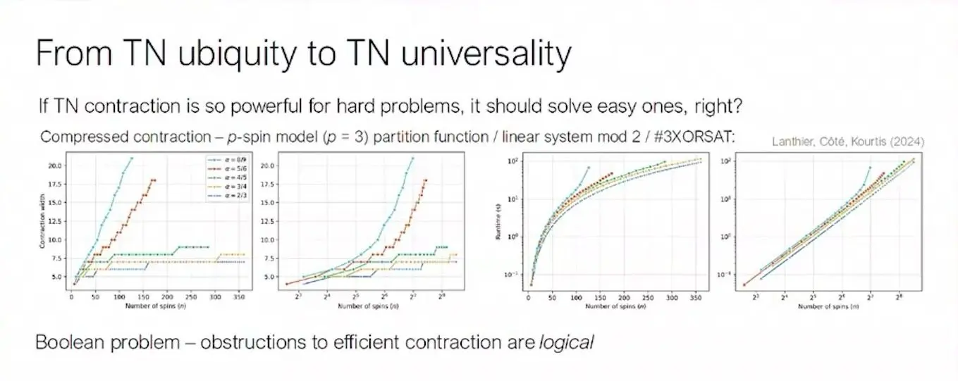
The fix copies old rules of logic. Kourtis showed a way to order the sums that copies the Davis-Putnam method of the 1960s, along with a tensor form of Gaussian elimination. Together they spot when a Boolean problem is in P, the class of easy problems, and then solve it in polynomial time even with its structure hidden. Kourtis named Clifford circuits as the next target.

Clifft runs full magic state cultivation on 463 qubits

Brad Chase of the Unitary Foundation presented Clifft, released in April 2026. Its target was cultivation, a protocol from Craig Gidney and colleagues in 2024. It makes the special states that fault-tolerant machines need for T gates. Those gates rule out Stim, the fast simulator for Clifford circuits, so the first paper used easier gates as a stand-in and worked out the rest from the trend.

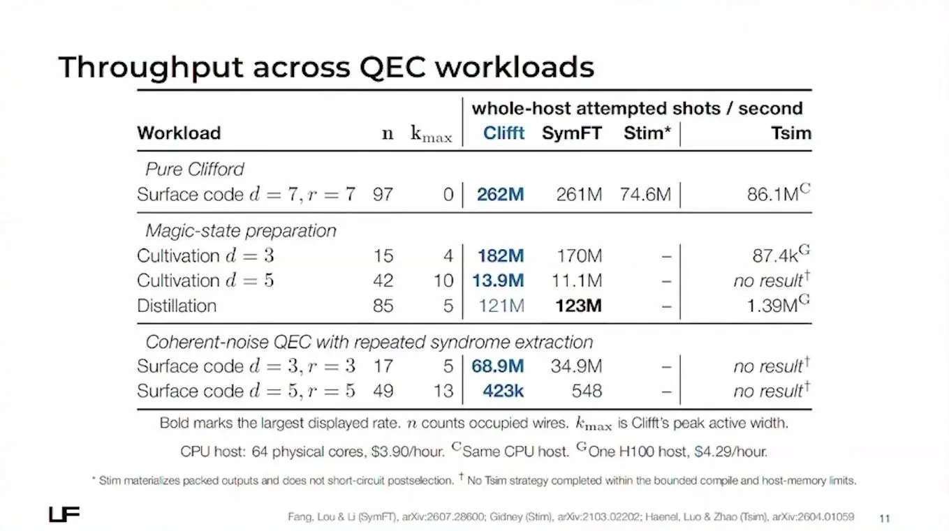
Clifft keeps a table for the Clifford gates seen so far and a state vector for only the few active qubits. Each non-Clifford turn can double that vector. Each measurement halves it. On 16 cores it ran full cultivation on 463 qubits at about 320,000 shots a second, for almost 400 billion shots in all, and GPU versions show little speed-up so far because the CPU version fits in cache.

Intel’s hybrid simulator runs about 30 times faster

Gian Giacomo Guerreschi of Intel presented a hybrid simulator, tested with CERN, the Technical University of Munich and the American University in Cairo. Intel’s simulator can turn many qubits at once for the cost of a one-qubit gate. But compilers break such turns into long ladders of CNOTs. So the hybrid folds each Clifford gate into a running record, called a Pauli frame, and puts each gate that is left on the full state in one go.

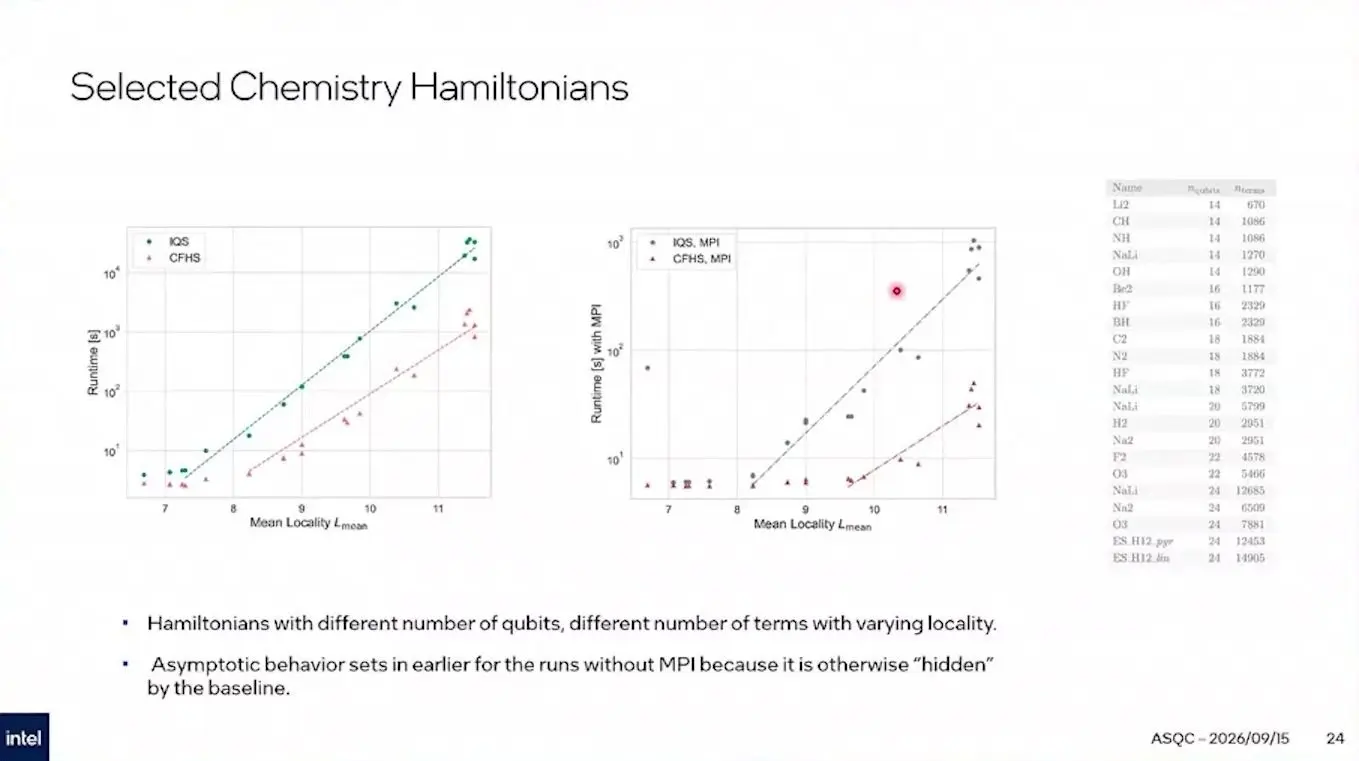
On made-up energy rules of 100 terms on 24 qubits, the run time fell about 30 times. Chemistry gained less. On chemistry problems of 14 to 24 qubits with up to almost 15,000 terms, the gain was around 20 times, and Guerreschi said that spreading the state over many nodes needs no extra traffic between them.

NVIDIA’s libraries run IBM’s utility test up to 178 times faster

Dmitry Lyakh, principal system software engineer for quantum at NVIDIA and a workshop organiser, toured the five cuQuantum libraries that other simulators call. One, cuPauliProp, tracks a measured value as a sum of Pauli strings and pushes it back through the circuit. It ran IBM’s 127-qubit utility test of 2023 up to 178 times faster on a DGX B200 than on a Xeon chip. That gap starts at 64 times.

cuStabilizer was quoted at two to three orders of magnitude faster than Stim at drawing a million shots. cuDensityMat, which solves a device’s equations at the pulse level, reached a space of 2 to the 40 states on 1,024 H100 cards at about 73 percent parallel efficiency. A Sherbrooke case reached 655,360,000 states on eight GPUs in 85.3 seconds.

ExtraFerm cuts chemistry error by up to 54 percent

Zack Hassman of the University of Chicago presented a paper with Oliver Reardon-Smith, Gokul Subramanian Ravi, Frederic Chong and Kevin Sung. ExtraFerm gives the odds of one chosen bit string. It works on circuits of matchgates, which a classical computer handles well, plus a few phase gates that add the hard part. Its cost stays small when those phase angles are small.

The team used it once, at the start of IBM’s sample-based diagonalisation, to rank bit strings and seed the first step. With 100,000 samples per point on an IBM Heron processor, energy error fell by up to 54 percent for a 60-qubit hydrogen chain and up to 18 percent for a 52-qubit nitrogen circuit. The extra runtime was under 2 percent, though the results were still short of chemical accuracy.

Compression takes a state-vector simulator to 56 qubits

Satoshi Imamura of Fujitsu Research presented a paper with Haruto Fujii, Nozomi Aoki, Akihiro Tabuchi, Ryuta Kawano and Akihiko Kasagi. A full state of n qubits holds 2 to the n numbers of 16 bytes each. At 50 qubits that is 16 petabytes. QompSim builds on the Qulacs simulator. It packs blocks of the state with a lossy squeeze and keeps a block of zeros as an empty pointer that each gate skips.

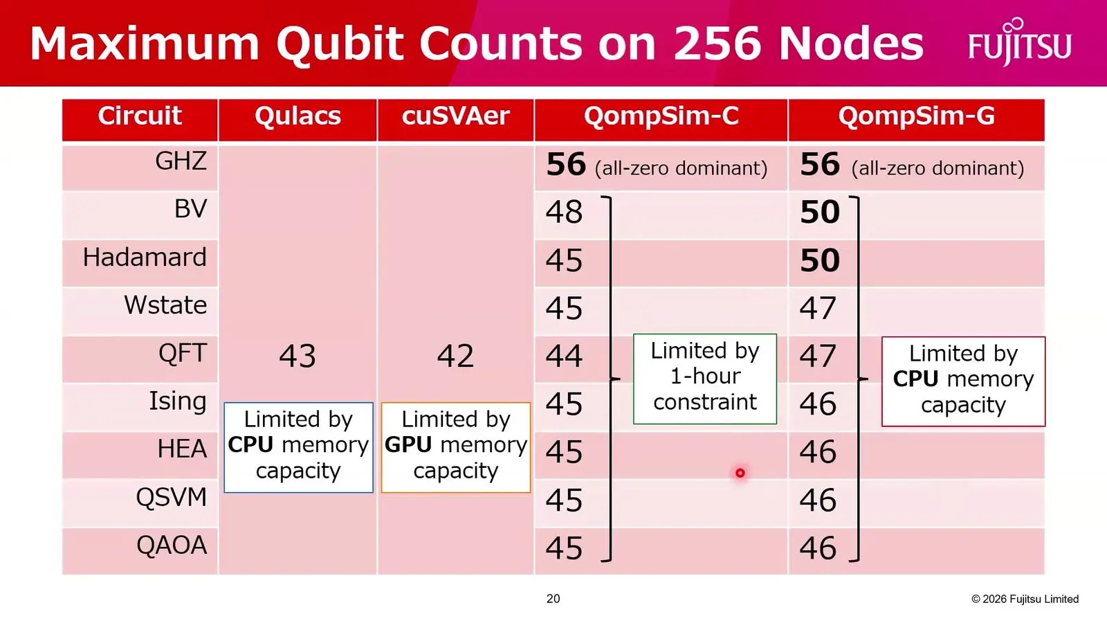
On 256 nodes of the ABCI-Q supercomputer, plain Qulacs topped out at 43 qubits. QompSim reached 56 on a GHZ circuit, where nearly every amplitude is zero, and 44 to 50 on eight other circuits, with fidelity near 0.99. It has a cost. On an Ising circuit with uneven amplitudes it ran slower, and Imamura said so openly.

Sdim simulates qudit codes seven orders of magnitude faster

Adeeb Kabir of Rutgers University presented a paper with Steven Nguyen, Sohan Ghosh, James Keppens, Tijil Kiran, Yipeng Huang, Isaac Kim and Bart Sorée. Qudits have d levels instead of two. Kabir said they may help error correction but had no tool to test their codes at scale. Sdim, named after the qubit simulator Stim, tracks the state as a table of integers and allows only Clifford gates.

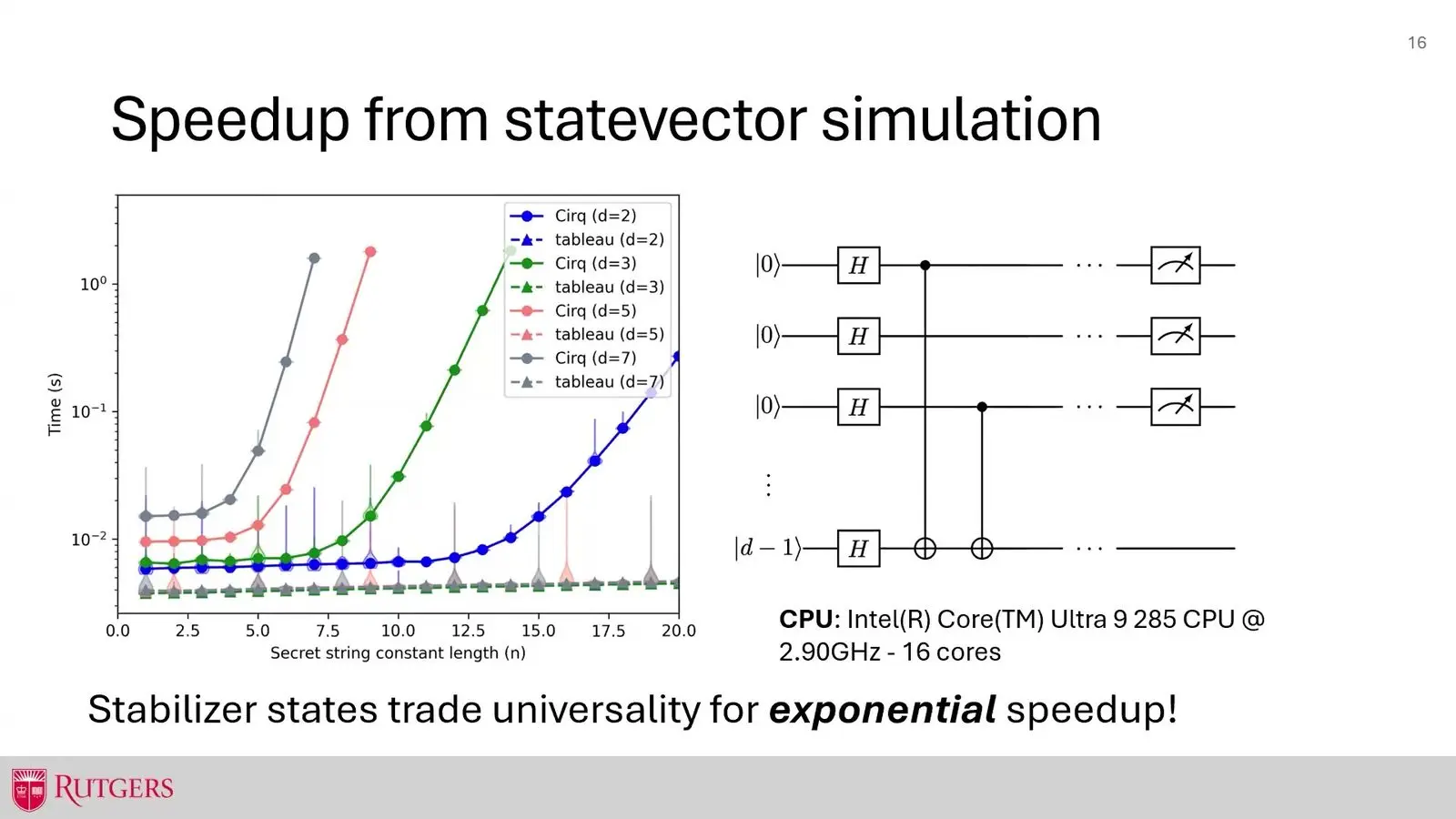
The table grows in step with the number of qudits and does not change with the dimension at all. The case study was a five-qutrit code, a three-level version of the five-qubit perfect code, and Sdim reran its threshold study seven orders of magnitude faster than a state-vector tool. Kabir said systems of 150 to 200 qudits run on a laptop.

Reusing shared openings speeds batches up to 33-fold

Tim Littau of Delft University of Technology presented a paper with Rihan Hai. Sweeps, repeated noisy shots and cycles of error correction often share the same opening, and QuWARP, a planner on top of the Qrack simulator, runs that opening once and hands the stored state to each branch. The trick comes from the planners that run database queries.

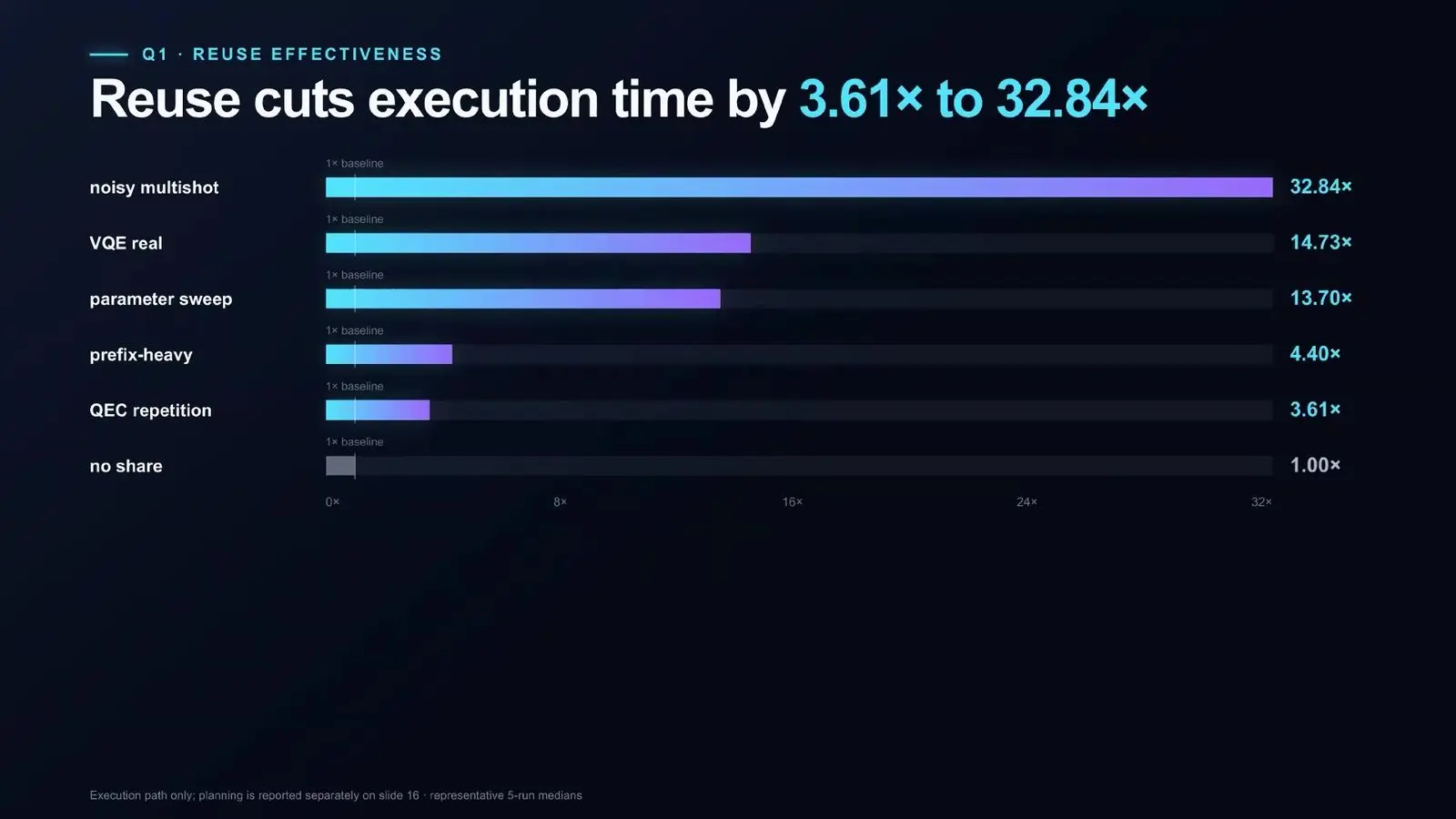
Speed-ups ran from 3.61 times on a repetition code to 32.84 times on noisy runs of many shots. Questioners called the test circuits too small. Littau said runs at 35 qubits on a cluster gave three to four times, and accepted that circuits with no exact shared structure gain nothing from the planner.

What it means for buyers, funders and reporters

Here is a rule for anyone who reads quantum claims for a living. Treat a claim of advantage as on hold until a classical group has tried to break it. Ask for the raw data behind any one score, and ask what a result costs for the fidelity it gives, just as Shinde’s ranking did when it put price next to quality. One funder’s version of that habit is the DARPA Quantum Benchmarking Initiative.

The auditors can be wrong too. Ali Javadi-Abhari of IBM Research said two leading classical methods disagreed with each other on a 56-qubit echo test, while mitigated runs on different IBM chips agreed. The hardware is improving, and some of the H2 results may well survive a classical attack when one comes, as one will for every claim in this guide. Mandrà’s simulation of a Quantinuum run is the model, an ordinary computer reading a quantum machine’s record and finding the error. For now the auditors hold the pen.