
Quantum computing crossed three lines in eighteen months that change what a basics article has to be. Google’s Willow chip ran error correction below the surface-code threshold for the first time. NIST published the first standardised post-quantum cryptography algorithms (FIPS 203/204/205) and bank CISOs started costing migrations.
Quantinuum filed to IPO and Atom Computing brought 1,200-plus qubits online, while IonQ paid $1.075B for Oxford Ionics, the largest pure-play quantum-hardware acquisition ever recorded. The quantum computing basics have shifted under everyone's feet, and most explainers on the open web have not kept up.
I have read about a hundred quantum computing basics pages in the last four years. The good ones get the physics roughly right but lose the plot on the engineering: Schrödinger's-cat metaphors that do not survive contact with a real qubit, five-modality lists with no guidance on which to actually try first, and a vague vendor pitch tacked onto the end.
This is the piece I wish I had been handed on day one: what a qubit really is, how superposition and entanglement combine inside an actual circuit, which of the six commercial modalities are worth your time in 2026, what the performance numbers really mean once you cut through the marketing, and the four problem categories where quantum machines genuinely beat classical computers, versus the much larger set where they do not. The goal is to give you the working mental model that lets you read industry announcements without being misled by marketing language.
What is quantum computing?
Classical computers represent information as bits, each of which is either zero or one. Every operation a CPU performs ultimately reduces to deterministic transformations on those bits. Quantum computers represent information as qubits, which can occupy a continuum of states between zero and one (a superposition) and which can become correlated with each other in ways that have no classical analogue (entanglement). The same Boolean abstraction that classical software is built on does not capture what a quantum machine does in the inner loop.
The field traces back to Richard Feynman’s 1981 observation that simulating quantum mechanics on a classical computer requires exponential resources in the number of particles, and that a computer made out of quantum components could in principle simulate quantum mechanics efficiently. John Preskill at Caltech has a memorable explainer of this same intuition aimed at a 9-year-old if you want the gentlest possible introduction.
Peter Shor turned the observation into a concrete commercial problem in 1994 by publishing a quantum algorithm that factors large integers in polynomial time, breaking the cryptographic assumption that protects most internet traffic. The intervening three decades have been about building the hardware to actually run Shor’s algorithm at problem sizes that matter, and the broader quantum computing basics around it – our scientific prelude to quantum computing covers the prehistory in more depth.
A brief history of quantum computing (Feynman 1981 to today)
Knowing the timeline matters because the major architectural decisions in 2026 hardware were made in response to specific historical events, and you can read the modern landscape much more cleanly if you know which of those events still constrains it. The threshold theorem alone explains why every serious quantum-error-correction roadmap targets 99% physical gate fidelity rather than some other number.
| Year | Milestone | Why it mattered |
|---|---|---|
| 1981 | Feynman’s Caltech lecture | Argued that simulating quantum mechanics on classical computers takes exponential resources, motivating the entire field. |
| 1985 | Deutsch’s universal quantum computer | First formal model of a quantum Turing machine; proved that quantum circuits can compute everything classical circuits can plus more. (See our profile of David Deutsch.) |
| 1994 | Shor’s factoring algorithm | Polynomial-time factoring of large integers; turned quantum computing from a curiosity into a national-security priority overnight. |
| 1996 | Grover’s search algorithm | Quadratic speedup for unstructured search; the second canonical quantum-advantage proof. |
| 1998 | First 2-qubit NMR demonstration | Chuang and colleagues ran Grover’s algorithm on a 2-qubit nuclear-magnetic-resonance device, the first running quantum algorithm. |
| 2007 | D-Wave Orion launches | First commercial quantum computer (a 16-qubit annealer); started the commercial era despite ongoing arguments about whether annealing counts as quantum advantage. |
| 2016 | IBM Quantum Experience launches | First publicly-accessible cloud quantum computer; the moment quantum computing became something a developer could actually try without being a physics PhD. |
| 2019 | Google Sycamore quantum supremacy | 53-qubit superconducting machine demonstrated a sampling task in 200 seconds that Google estimated would take a classical supercomputer 10,000 years; first formal quantum-advantage demonstration. |
| 2022 | IBM Osprey 433 qubits + Xanadu Borealis | IBM crossed 400 qubits on superconducting; Xanadu’s Borealis demonstrated photonic quantum advantage on Gaussian boson sampling. |
| 2023 | IBM coined "quantum utility" | Nature paper introducing the term reframed the procurement story from waiting for advantage to deploying for utility today. |
| 2024 | Google Willow 105 qubits with QEC below threshold | First experimental demonstration of error correction below the surface-code threshold, opening the path to fault-tolerant scaling. |
| 2024 | NIST publishes FIPS 203/204/205 | First standardised post-quantum cryptography algorithms; enterprise PQC migration begins in earnest. |
| 2025 | IonQ 99.99% two-qubit fidelity + Atom Computing 1,200+ qubits + IonQ acquires Oxford Ionics for $1.075B | The trapped-ion fidelity record, the largest neutral-atom system, and the largest single trapped-ion acquisition all in one calendar year. |
| 2026 | Quantinuum files for IPO; Xanadu trades on NASDAQ | Pure-play quantum-computing companies become commodity public-market trades; the modality enters mainstream investor portfolios. |
Two patterns matter here. First, the gap between Shor (1994) and the first useful Shor implementation is now over thirty years, which is the right cadence for thinking about how long fault-tolerant practical computing will take from today. Second, the commercial era only really started in 2016 with IBM’s cloud, which means most of the production engineering knowledge in the field is less than ten years old. Anyone telling you the basics are settled is forgetting how recent everything is.
The four quantum primitives
Four physical phenomena anchor every quantum algorithm. Knowing them is the price of admission to understanding the quantum computing basics in any depth.
Superposition
A single qubit can occupy a linear combination of the |0⟩ and |1⟩ basis states, parameterised by two real numbers (a probability amplitude and a phase). N qubits in superposition span 2ⁿ basis states simultaneously, which is what gives quantum computers their structural ability to evaluate many computational paths in parallel before measurement collapses the result back to a single classical answer.
Entanglement
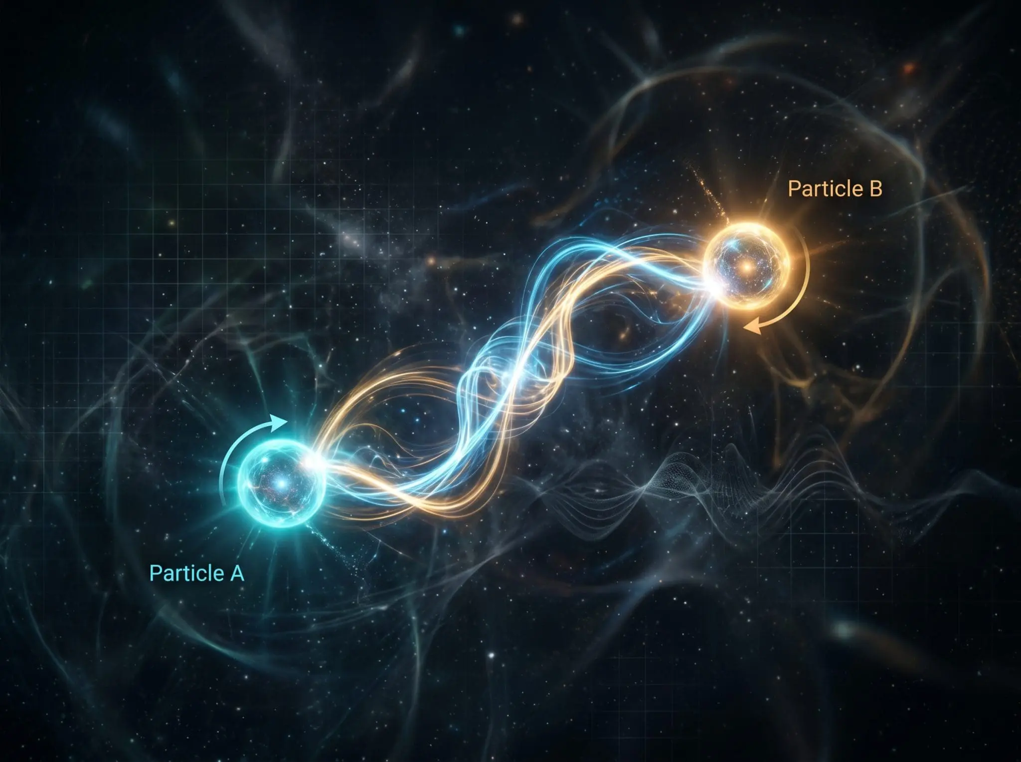
Two or more qubits can be correlated in a way that the state of one cannot be described independently of the other. Measuring one entangled qubit instantly determines the measurement statistics of the other, regardless of distance. Entanglement is the resource that distinguishes quantum computing from classical probabilistic computing and is the reason quantum networks (covered in our top quantum networking companies guide) are an engineering field in their own right. The no-cloning theorem is what makes entanglement-distribution networks possible: the same property that prevents copying a quantum state mid-flight gives QKD its security guarantee.
Interference
Quantum amplitudes are complex numbers, and they add constructively or destructively. Quantum algorithms are designed so that the amplitudes of correct answers add up while the amplitudes of incorrect answers cancel out, leaving a measurement that reads the right answer with high probability. The Quantum Fourier Transform is the canonical example: it sets up exactly this constructive-destructive pattern across an exponentially large state space and is the engine behind Shor’s algorithm and quantum phase estimation. Recent QZ coverage of nearly-perfect interference at chip scale shows how serious modern QC engineering takes the need for clean interference patterns.
Decoherence
Real quantum systems do not stay quantum forever. Stray electromagnetic fields, thermal vibrations, and stray photons all cause the qubit’s quantum state to leak into the surrounding environment, randomising the phase and probability amplitudes. The time over which this happens is the coherence time, and it is the dominant engineering constraint on every qubit modality. Every other component in a quantum machine (cryostats, vacuum chambers, electromagnetic shielding, fast control electronics) exists to push the coherence time as far as possible.
How the four primitives work together
The reason I keep coming back to these four primitives in the same order is that they describe a complete algorithmic pipeline. You start with a register of qubits initialised in a definite state, apply gates that put them into a deliberate superposition, apply more gates that entangle them according to the structure of the problem you are solving, and then design the rest of the circuit so that interference makes the amplitudes of the correct answers add up while the amplitudes of incorrect answers cancel out.
Decoherence is the hostile force the entire engineering stack is fighting: every nanosecond the algorithm runs, the environment is trying to leak away the phase information that interference depends on. A working quantum algorithm is one that finishes before decoherence wins.
The five components of a quantum computer

Every quantum machine, regardless of modality, has the same five layers. The labels differ between vendors but the underlying stack is identical from superconducting transmons to neutral atoms to silicon spins.
The physical two-level systems that store quantum information. Implemented as superconducting circuits, trapped ions, neutral atoms, photons, or semiconductor spins.
Reversible operations that transform qubit states. Single-qubit gates (X, Y, Z, H, S, T) and two-qubit entangling gates (CNOT, CZ) form a universal set.
Sequences of gates applied to qubits. The circuit depth determines how long the algorithm needs to run before decoherence destroys the state.
Projective readout of each qubit at the end of the circuit, returning a classical bitstring with a probability determined by the final quantum state. The measurement also collapses the state, which is why every quantum algorithm has to be designed around getting useful information out in a single shot.
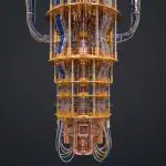
The supporting infrastructure: cryostats, lasers, vacuum chambers, control electronics, and the room-temperature classical compute that orchestrates the run. The supporting layer is where most of the modality-specific cost lives, which is why a 1,000-qubit superconducting machine and a 1,000-qubit neutral-atom machine look completely different in person.
The terminology is unfamiliar at first; our glossary of the 20 quantum computing terms you need to know covers the rest of the vocabulary. For deeper reading, our curated list of the best quantum computing books includes the canonical Nielsen and Chuang textbook plus newer beginner-friendly overviews, and the 2024 Nature review on quantum machine learning and quantum computing basics is the best single-source academic overview.
Hello, Bell State: a 10-line working example
The simplest non-trivial quantum circuit is a Bell-state preparation: a Hadamard gate puts the first qubit in superposition, then a CNOT entangles it with the second. Measuring both qubits produces correlated 00 and 11 outcomes with equal probability, and never 01 or 10, which is the experimental signature of entanglement. Run this on the IBM Quantum Platform Aer simulator or any IBM, IonQ, or Quantinuum backend through Qiskit Runtime:
from qiskit import QuantumCircuit, Aer, execute
qc = QuantumCircuit(2, 2)
qc.h(0) # Hadamard puts qubit 0 in superposition
qc.cx(0, 1) # CNOT entangles qubit 0 with qubit 1
qc.measure([0, 1], [0, 1])
backend = Aer.get_backend('qasm_simulator')
counts = execute(qc, backend, shots=1024).result().
print(counts) # {'00': ~512, '11': ~512}, never '01' or '10'Run this and you have demonstrated entanglement in ten lines. The Bell state is the foundational primitive behind quantum teleportation, superdense coding, and the swap-test kernel computations that drive quantum machine learning algorithms.
The famous quantum algorithms in plain English
Most quantum computing basics articles list quantum algorithms as a vocabulary table and move on. That undersells them. Each of the famous algorithms reveals something specific about why quantum machines do what they do, and knowing them is the difference between reading the field and understanding it.
Shor’s algorithm (1994): factoring large integers
The algorithm that started the commercial field. Shor showed that factoring an N-bit integer takes polynomial time on a quantum computer (specifically O(N³) gates with the standard implementation), where the best classical algorithm (the General Number Field Sieve) takes sub-exponential time. Since RSA encryption rests on the assumption that factoring is hard, Shor’s algorithm at scale would break RSA. This is the threat behind the entire post-quantum cryptography migration that NIST started in 2016 and standardised in 2024. The algorithm uses Quantum Phase Estimation to find the period of a function modular over the input, then classical post-processing extracts the factors. Recent QZ coverage on SHA-256 quantum attack vulnerability shows how the cryptographic threat now extends beyond pure RSA.
Grover’s search algorithm (1996): unstructured search
Given an unstructured database of N items, classical search needs O(N) queries on average to find a target. Grover’s algorithm needs only O(√N) queries, a quadratic speedup. The algorithm works by amplitude amplification: it creates a superposition over all N items, applies a phase flip to the target, then reflects the amplitudes around their mean to amplify the target. After roughly √N iterations, measuring returns the target with high probability. The speedup is real but quadratic rather than exponential, which limits the practical impact compared with Shor.
Variational Quantum Eigensolver (VQE)
The workhorse of near-term quantum chemistry. VQE prepares a parameterised quantum state that approximates the ground state of a chemical Hamiltonian, then iteratively adjusts the parameters with a classical optimiser to minimise the measured energy. The quantum machine evaluates the energy expectation; the classical machine drives the optimisation. VQE runs on noisy intermediate-scale (NISQ) hardware today and is the algorithm behind most of the production quantum-chemistry workloads at BASF, Boehringer Ingelheim, BMW, and Roche.
Quantum Approximate Optimization Algorithm (QAOA)
The variational answer to combinatorial optimisation. QAOA encodes a QUBO problem (Quadratic Unconstrained Binary Optimisation) into a cost Hamiltonian, then alternates applications of the cost Hamiltonian and a mixing Hamiltonian for p layers. Increasing p tightens the approximation. QAOA at p=1 is competitive with classical heuristics on some problems and uncompetitive on others; the empirical landscape is the most studied and most contested of any near-term quantum algorithm.
HHL algorithm (Harrow-Hassidim-Lloyd)
The 2009 algorithm that solves linear systems Ax = b in time logarithmic in N (the number of variables) under specific conditions on the matrix structure. HHL is the engine behind many proposed exponential-speedup machine-learning algorithms; QZ has covered HHL-style approaches accelerating fluid-dynamics simulation and QKML for materials discovery as recent applications. The dequantisation literature (Tang 2018 and follow-ups) has shown that classical algorithms can match HHL on some of those proposed advantages, which is why the field treats HHL-derived speedups with more scepticism in 2026 than in 2014.
Quantum Phase Estimation (QPE)
Not a flashy headline algorithm but a foundational primitive: QPE estimates the eigenvalue (the phase) corresponding to an eigenvector of a unitary operator. Shor’s factoring is QPE applied to a specific modular-arithmetic unitary. Quantum chemistry’s exact diagonalisation methods use QPE. Many fault-tolerant algorithms reduce to QPE plus state preparation. Worth knowing because it appears everywhere in the literature.
Quantum Fourier Transform (QFT)
The quantum analogue of the Discrete Fourier Transform, computable in O(n²) gates on n qubits compared with O(n·2ⁿ) for classical FFT. QFT is the engine inside QPE, Shor’s algorithm, and many quantum-signal-processing routines. Once you understand QFT, you understand why so many quantum algorithms feel like they reduce to the same primitive: most of them do.
The six commercial qubit modalities
Six distinct hardware approaches are commercially deployed in 2026, each with a different physics and a different commercial roadmap. Knowing these is the most practical part of the quantum computing basics for anyone evaluating vendor claims.
| Modality | Largest commercial system | Key vendors |
|---|---|---|
| Superconducting transmon | IBM Heron R2 (156 qubits) | IBM, Google, Rigetti, IQM, OQC, SeeQC |
| Trapped ion | Quantinuum H2 (56 qubits, 33.5M QV) | IonQ, Quantinuum, AQT, Oxford Ionics, Universal Quantum, eleQtron |
| Neutral atom (Rydberg) | Atom Computing AC1000 (1,200+ qubits) | QuEra, Pasqal, Atom Computing, Infleqtion, planqc |
| Photonic | Xanadu X-series (hundreds of modes) | PsiQuantum, Xanadu, Quandela, ORCA, QuiX, Aegiq |
| Silicon spin | Quantum Motion CMOS (research scale) | Quantum Motion, Diraq, Equal1, Silicon Quantum Computing |
| Quantum annealing | D-Wave Advantage2 (4,400+ qubits) | D-Wave |
Each modality is covered in depth in a dedicated guide. The trapped-ion modality holds the gate-fidelity record at 99.99%; the neutral-atom modality has scaled fastest on qubit count; the photonic modality runs at room temperature without dilution refrigerators. The full lineup across all modalities is summarised in our top quantum hardware companies guide.
Quantum error correction explained
Every modality faces the same brutal arithmetic. Two-qubit gates have 99.5-99.99% fidelity in the best 2026 hardware, which sounds great until you realise that a useful Shor’s-algorithm circuit needs trillions of gates. At 99.99% fidelity, the probability that all trillion gates execute correctly is essentially zero. Quantum error correction (QEC) is the family of techniques that fixes this by encoding one logical qubit into many physical qubits, with the redundant qubits used to detect and correct errors as they happen.
Physical qubits versus logical qubits
A physical qubit is what the hardware actually implements: a single transmon, a single trapped ion, a single neutral atom in an optical tweezer. A logical qubit is an error-corrected abstraction built on top of many physical qubits. The simplest non-trivial QEC code (the [[7,1,3]] Steane code) encodes one logical qubit into seven physical qubits and corrects any single-qubit error. The currently-favoured surface code uses thousands of physical qubits per logical qubit at realistic error rates. The published quantum logical-qubit leaderboard tracks the count of logical qubits demonstrated on each platform.
The threshold theorem
The single most important result in QEC. The threshold theorem (Aharonov-Ben-Or 1997 and refinements) proves that if the per-gate error rate falls below a fixed threshold (roughly 1% for the surface code), then arbitrarily long quantum computations can be made arbitrarily reliable by adding more physical qubits per logical qubit. Above the threshold, errors compound faster than QEC can correct them and the computation diverges. Below the threshold, error correction wins and you can scale to fault tolerance. Modern hardware fidelities (99.5%-99.99% on two-qubit gates) put us comfortably below the surface-code threshold, which is why the field is now scaling rather than searching for a better gate.
Why we need a million physical qubits
The hard arithmetic. To run Shor’s algorithm at RSA-2048 with a useful success probability, you need roughly 4,000 logical qubits running circuits trillions of gates deep. At today’s two-qubit error rate of 99.99%, the surface code needs around 1,000 physical qubits per logical qubit to deliver the necessary suppression. 4,000 logical qubits times 1,000 physical-per-logical equals 4,000,000 physical qubits. Drop the error rate to 99.999% (which Quantinuum and IonQ are targeting) and the ratio drops to maybe 100:1, bringing the requirement down to 400,000 physical qubits. Hardware roadmaps from IBM, IonQ, Quantinuum, and PsiQuantum all target this regime by the early 2030s.
What broke the surface-code threshold in 2024
Google’s December 2024 Willow result was the first experimental demonstration that adding more physical qubits to a surface-code patch actually decreased the logical error rate (rather than increasing it as had been the case in earlier smaller demonstrations). That below-threshold demonstration was the result the field had been chasing for fifteen years and is the reason the 2030 fault-tolerant timelines are now considered aspirational rather than fantastical. Atom Computing and IBM Quantinuum demonstrated similar threshold-crossing results in 2024-2025 on different platforms. Riverlane’s 2026 predictions for QEC are the most concrete published timelines, and the qLDPC codes literature covers the next-generation alternatives to surface codes that may compress the physical-qubit overhead further.
How quantum performance is measured
Five metrics dominate the published quantum-performance literature, and they capture different aspects of what makes a quantum machine useful. The metrics are not interchangeable, and a vendor leading on one metric is often quietly behind on another.
Qubit count
The headline marketing number. Useful but partial: 1,200 noisy neutral-atom qubits do not necessarily outperform 156 high-fidelity superconducting transmons on the same workload. The number that matters for fault-tolerant computing is logical-qubit count rather than physical-qubit count, and the published quantum logical-qubit leaderboard tracks that more honestly than headline announcements.
Quantum Volume (QV)
An IBM-introduced single-number metric that combines qubit count, gate fidelity, and connectivity. A QV of 2ⁿ means the machine can run depth-N circuits on N qubits with high enough fidelity to produce useful output. Quantinuum holds the published record at 33.5 million.
Gate fidelity and error rates
The probability that a gate operation produces the intended result. Single-qubit gates routinely exceed 99.9% on production hardware; two-qubit gates are the limiting factor and now reach 99.5-99.99% across the leading modalities. IonQ’s announcement of 99.99% two-qubit fidelity in 2025 was the highest published number on any platform. Below 99% gate fidelity, fault-tolerant computing is essentially out of reach because error correction needs more correctable cycles than the gates can deliver.
Coherence time
The duration over which a qubit retains its quantum information before decoherence destroys it. T1 (relaxation) and T2 (dephasing) are the standard sub-metrics. Trapped-ion qubits have the longest coherence times (seconds to minutes); superconducting transmons run at hundreds of microseconds; neutral atoms sit between. Coherence time directly limits the maximum useful circuit depth.
Gate speed and circuit depth
How fast each operation runs and how many can fit inside a coherence time. Superconducting transmons have the fastest gate times (tens of nanoseconds) which compensates for shorter coherence; trapped ions are slower per gate but stay coherent much longer. The product of gate speed and coherence time roughly determines the deepest circuit a machine can run.
Layer fidelity
The newest performance metric in the IBM stable, layer fidelity captures the success probability of a single layer of parallel two-qubit gates across an entire processor, which is more discriminating than per-gate fidelity for production-scale workloads. IBM publishes layer-fidelity numbers alongside Quantum Volume on the Heron R2 system, and the metric has begun to displace single-gate fidelity as the procurement-grade benchmark for fault-tolerant-class workloads. Track this one if you are deciding which of two superficially-similar machines to spend a budget on.
Quantum versus classical at a glance
| Property | Classical computer | Quantum computer |
|---|---|---|
| Information unit | Bit (0 or 1) | Qubit (superposition of 0 and 1) |
| State space (N units) | 2ⁿ values, one at a time | 2ⁿ amplitudes, all at once |
| Gate model | Boolean logic (AND, OR, NOT) | Unitary gates (H, X, CNOT, T) |
| Read-out | Deterministic | Probabilistic (one shot per circuit run) |
| Best at | Spreadsheets, web servers, training LLMs | Chemistry simulation, optimisation, factoring, sampling |
| Worst at | Simulating quantum mechanics | General-purpose computing |
| Energy use | Watts to kilowatts | Kilowatts to megawatts (cryogenics dominate) |
The takeaway most beginner pieces miss: quantum computers do not replace classical computers, they augment them on specific structured workloads. The dominant 2026 deployment pattern is hybrid: classical orchestration calling out to a quantum kernel computation, then back to classical post-processing. Anyone who tells you otherwise is selling something.
When quantum computing actually wins
The quantum-advantage question is the hardest one in the quantum computing basics. The honest 2026 answer is that quantum machines win on specific structured problems and remain uncompetitive on general-purpose tasks like spreadsheets, web servers, or training large language models. Four problem categories cover most of where the wins actually appear.
Optimisation
Combinatorial optimisation problems (route planning, portfolio allocation, scheduling) map cleanly to QUBO formulations that quantum annealers and gate-model variational algorithms can attack. D-Wave Leap and the Quantum Approximate Optimisation Algorithm (QAOA) are the dominant approaches, and the empirical picture is mixed: classical heuristics beat QAOA on the binary paint-shop problem, while recent benchmarking on real-world tasks shows real wins on structured instances. Where it works, it really works; where it does not, classical baselines remain competitive.
Simulation of physical systems
The original Feynman use case. Simulating quantum chemistry, materials, and condensed-matter systems on classical computers requires exponential resources; quantum machines can do it in polynomial resources for problems large enough to matter. This is the use case with the strongest theoretical foundation and is the primary near-term target for IBM, Google, IonQ, Quantinuum, Pasqal, and the broader quantum-chemistry research community.
Machine learning and pattern recognition
Quantum kernel methods, variational quantum classifiers, and quantum neural networks form the field of quantum machine learning. The empirical picture is the most contested in the basics: on quantum-native data (chemistry samples, sensor outputs) the wins are real; on classical tabular data the picture is mixed. The quantum k-means clustering walkthrough shows the swap-test primitive in action on a worked example.
Search and sampling
Grover’s algorithm gives a quadratic speedup for unstructured search, and quantum sampling can produce distributions that classical machines cannot easily reproduce. The 2019 Google Sycamore and 2022 Xanadu Borealis quantum-advantage demonstrations both used sampling tasks with no commercial value but with provable separation from classical computation, which set the precedent that the wins are real even if they are not yet useful.
Use cases worth tracking in 2026
Cryptography and security
Shor’s algorithm threatens RSA, ECC, and Diffie-Hellman key exchange when sufficiently large fault-tolerant quantum machines exist. The cryptographic community is mid-migration to post-quantum cryptography, and the harvest-now-decrypt-later threat model is driving 2026 procurement timelines that did not exist three years ago.
Drug discovery and chemistry
Variational quantum eigensolvers running on small molecules with classical-quantum hybrid optimisation, then scaling toward quantum-neural-network surrogate models for protein folding and drug binding. Boehringer Ingelheim, BASF, BMW, and Roche all have active programmes; the Pasqal-Aramco-IBM quantum-centric supercomputing partnership is the largest published industrial chemistry deployment.
Financial modelling and risk
Portfolio optimisation through QAOA-style variational circuits, derivative pricing through quantum amplitude estimation, and credit-risk scoring through interpretable quantum neural networks. JPMorgan Chase, HSBC, Goldman Sachs, and BNP Paribas all publish Qiskit Runtime and Pasqal benchmarks; the 2026 pattern is multi-cloud benchmarking through one of the major quantum cloud providers.
Artificial intelligence
Hybrid quantum-classical neural networks, quantum-inspired tensor methods (matrix product states, projected entangled pair states), and quantum reinforcement-learning policies. Multiverse Computing’s compression of large language models on superconducting hardware is the most-deployed example, and the top quantum software companies guide covers the broader stack.
Energy and materials
Battery chemistry, photovoltaic materials, and catalyst design through quantum-chemistry workloads on the same hardware that serves drug discovery. Quantinuum’s BMW partnership is the most-cited materials-science deployment, and Microsoft Azure Quantum Elements ships materials workloads as a managed service.
Real-world deployments (case studies)
The most useful way to ground the quantum computing basics is to look at what specific organisations are running on quantum hardware in production, what they are getting from it, and how they are paying for it. The list below covers the deployments that have been publicly documented through company announcements, regulatory filings, or peer-reviewed publications.
BMW + Quantinuum: materials science
BMW runs density-functional-theory calculations for new battery and catalyst materials on Quantinuum’s H-series trapped-ion systems through Microsoft Azure Quantum. The published 2025 results show measurable speedup on small-molecule active-space chemistry workloads, and BMW publicly committed to multi-year continued spending on Quantinuum hardware. The procurement story is hybrid: classical DFT runs the bulk of the workload, the quantum machine attacks the active-space subset where classical scaling falls over.
Pasqal + Aramco: Saudi Arabia’s first quantum computer
Pasqal delivered Saudi Arabia’s first 200-qubit neutral-atom quantum computer to Aramco under a partnership announced in November 2025. The deployment runs energy-sector chemistry workloads (catalysis, hydrogen-production reaction simulation) plus optimisation workloads for refinery scheduling. The on-premise machine plus Pasqal’s cloud access through the IBM Quantum Platform supercomputing partnership gives Aramco a hybrid stack that few customers have today.
JPMorgan Chase: portfolio optimisation
JPMorgan Chase has published a steady stream of quantum-finance papers since 2019, running QAOA-style portfolio optimisation, derivative pricing through quantum amplitude estimation, and credit-risk scoring through interpretable quantum neural networks on IBM Qiskit Runtime. The bank’s QC@JPMC team is one of the largest quantum-engineering groups inside any traditional finance firm, and the published benchmarks set the empirical standard for quantum-finance evaluation.
Boehringer Ingelheim + Google Quantum AI: drug discovery
Boehringer’s quantum-chemistry partnership with Google Quantum AI uses Sycamore-class hardware for variational chemistry on small drug-binding-pocket simulations, with classical-quantum hybrid optimisation driving the search. The deployment is research-grade rather than production drug-discovery yet, but the company has been one of the most consistent published case studies in pharma quantum computing.
D-Wave Leap customers: combinatorial optimisation
Mastercard runs fraud-detection and rewards-optimisation workloads on D-Wave Leap; Pattison Food Group runs supply-chain optimisation for grocery distribution; NTT DoCoMo runs cell-tower planning. D-Wave Leap is the longest-running production quantum-cloud service and has the highest count of paying enterprise customers running live workloads in 2026. The hybrid solvers (Constrained Quadratic Model, Discrete Quadratic Model, Nonlinear) handle problem instances that exceed pure-QPU capacity.
Multiverse Computing: LLM compression
Multiverse Computing’s CompactifAI service uses tensor-network methods (matrix product states) on IBM and IonQ hardware to compress large language models by 1.4-3% perplexity loss in exchange for substantial parameter reduction. The company has shown the technique on 156-qubit IBM Heron systems and continues to scale toward larger LLMs. This is one of the few production quantum-AI deployments that maps to a workload businesses already pay for.
Quantum utility versus quantum advantage
Two distinct claims confuse this part of the quantum computing basics. Quantum advantage is the formal demonstration that a quantum machine can do a specific task faster than the best known classical algorithm. The 2019 Google Sycamore experiment was the first commercially-meaningful quantum-advantage claim; Xanadu’s Borealis followed in 2022 with a photonic Gaussian-boson-sampling demonstration. Both have been partially dequantised by classical algorithms in subsequent years, which is the normal pattern and does not invalidate the original demonstrations.
Quantum utility is the weaker but more practical claim that a quantum machine can run useful real-world computations in regimes where classical methods are expensive. IBM’s 2023 Nature paper introducing the term framed it explicitly: not faster than classical, just useful enough to be worth running. Most 2026 commercial deployments target quantum utility rather than quantum advantage, and the procurement story has shifted from “wait for the breakthrough” to “deploy where it works today and scale as the hardware improves”.
Five common misconceptions worth dispelling
I have argued each of these out so many times that I will just put them in writing. Each point is the consensus position you will reach after talking to enough practitioners, even if the popular press still pushes a different framing.
1. "Quantum computers try every answer in parallel"
The most common misconception in beginner explanations. A quantum computer in superposition has access to amplitudes for all 2ⁿ basis states, but measurement collapses the state to a single outcome with probability determined by the amplitudes. You do not get to read out all 2ⁿ outcomes for free; you get one outcome per shot. The algorithmic skill is using interference to make the right answer have the highest amplitude before measurement. "Parallelism" is a misleading shortcut for "structured constructive interference across exponentially-many computational paths".
2. "Quantum mechanics is just probabilities"
Quantum mechanics is not classical probability theory with extra steps. Probability amplitudes are complex numbers, which means they can interfere destructively (cancel out) in ways probabilities cannot. Bell’s theorem rules out any local hidden-variable model that would let you describe quantum mechanics as classical probabilistic computing in disguise. The 2022 Nobel Prize in Physics was awarded to Aspect, Clauser, and Zeilinger for the experiments that closed the local-realism loopholes; this is settled physics.
3. "Quantum computers will replace classical computers"
They will not. Quantum computers are good at specific structured problems (chemistry simulation, optimisation, factoring, sampling) and uncompetitive on general-purpose tasks (running web servers, training large language models, manipulating spreadsheets). The 2026 deployment pattern is hybrid: classical orchestration calling out to a quantum kernel computation for the bottleneck step, then back to classical post-processing. Anyone selling you a quantum-only architecture for a general-purpose workload is selling something they should not.
4. "Quantum supremacy means quantum is now useful"
Quantum supremacy (or quantum advantage in the more recent terminology) is a formal computational-complexity claim: a quantum machine can do a specific task faster than the best known classical algorithm. The 2019 Google Sycamore demonstration was for a sampling task with no commercial value. Useful quantum computing (running real workloads that produce real value) is a different and weaker claim that IBM coined "quantum utility" in 2023. Most 2026 commercial deployments target utility rather than advantage.
5. "Quantum computers will break all encryption tomorrow"
They will not. The most-cited timeline for cryptographically-relevant fault-tolerant quantum computers (machines capable of running Shor’s algorithm at RSA-2048 scale) is 2030-2035 with significant uncertainty. The risk that matters today is the harvest-now-decrypt-later threat model: long-lived secrets recorded today can be decrypted retroactively when sufficiently capable hardware exists. The cryptographic community is mid-migration to post-quantum cryptography precisely to defuse this longer-horizon risk.
Current challenges and outlook
Three structural challenges remain. The QED-C industry consortium tracks the quantum computing basics ecosystem with quarterly status updates that frame these challenges in commercial terms, and the NIST Quantum Information Science programme publishes the federal-research roadmap alongside the FIPS 203/204/205 post-quantum cryptography standards. First, error correction overhead: the leading codes need roughly 1,000 physical qubits per logical qubit at current error rates, which means a million physical qubits to run a useful Shor’s-algorithm-class workload. Hardware roadmaps from IBM, Google, IonQ, Quantinuum, and PsiQuantum all target this regime by the early 2030s, but the timelines are aspirational rather than guaranteed. IBM Research’s published quantum roadmap is the most-cited public reference point for what an aggressive but plausible timeline looks like.
Second, software maturity: the developer tooling has improved enormously since 2019 but still lags classical software ecosystems by a wide margin. Qiskit, Cirq, PennyLane, Q#, and Classiq are the dominant stacks, and each has its own community, optimiser conventions, and hardware-backend integration story.
Third, the dequantisation question: every few months, classical algorithms catch up with previously-claimed quantum speedups. The honest 2026 outlook is that quantum machines have a structural advantage on specific problem classes and need to be deployed selectively, not as general-purpose accelerators. Anyone learning the quantum computing basics should treat marketing claims with the same scepticism they would apply to any frontier-technology pitch.
Hands-on: your first 30 minutes with the quantum computing basics
Concrete, sequential, and entirely free. If you finish this section you will have run a real quantum circuit on either a simulator or real hardware, and you will have a working development environment for everything else in the field.
Minute 0-10: Sign up and install
Register for an IBM Quantum Platform Open Plan account at quantum.ibm.com (free, with monthly time quotas; QZ profiled the platform’s switch to qBraid as the recommended notebook host). While that confirmation email arrives, install Qiskit locally with one pip command (pip install qiskit qiskit-aer qiskit-ibm-runtime) and Jupyter if you do not have it. Alternatively, register for a qBraid Lab account at qbraid.com, which gives you a managed Jupyter notebook environment plus pre-installed Qiskit, Cirq, PennyLane, and access to multi-vendor quantum hardware through one API. qBraid was IBM’s recommended replacement for the sunset Quantum Lab notebooks in November 2024, and it is the lowest-friction path from zero to running code in 2026.
Minute 10-20: Run the Bell state circuit
Open a Jupyter notebook, paste in the 10-line Bell-state code from earlier in this piece, and run it on the local Aer simulator. You should see roughly 512 counts of ’00’ and 512 counts of ’11’, with no ’01’ or ’10’ results (modulo shot noise). Congratulations, you have demonstrated entanglement in your first ten minutes. Then change the backend to a real IBM machine via Qiskit Runtime sessions, resubmit, and watch the same result come back from quantum hardware in a few minutes (queue time included).
Minute 20-30: Try variational classification
Now stretch. Open the Qiskit Machine Learning tutorial on variational quantum classifiers, run the iris-dataset notebook end-to-end, and compare the trained quantum classifier’s accuracy against scikit-learn’s logistic regression on the same data. The point is not to win on accuracy; the point is to feel the full classical-quantum hybrid loop: classical optimiser driving quantum circuit evaluation in the inner loop, parameter updates, convergence. The quantum k-means clustering walkthrough covers a similar workflow in clustering form, and the quantum machine learning pillar lays out the broader algorithmic landscape.
Where to go next
The IBM Quantum Learning resources, the PennyLane tutorials, and the Microsoft Quantum Katas are the three best free curricula in 2026. Pair them with the Nielsen and Chuang textbook for the foundational theory and one of the newer practitioner-focused books from our curated reading list. If you want to go deeper into the quantum software stack, the quantum cloud provider landscape, or any of the six commercial qubit modalities, the QZ pillar cluster is built to support that exact research path. Vocabulary-builders worth bookmarking: Top 20 quantum computing terms, Top 20 Cirq terms, and Top 20 quantum cloud computing terms.
Frequently asked questions
What are the quantum computing basics in one paragraph?
Quantum computers represent information as qubits that can exist in superposition (a continuous combination of zero and one states) and become entangled with each other (correlations that have no classical analogue). They use sequences of quantum gates inside circuits to manipulate this information, then measure the qubits at the end to read out a classical bitstring. The hardware comes in six commercial modalities (superconducting transmons, trapped ions, neutral atoms, photonic, silicon spin, quantum annealing) and is rated on metrics like qubit count, Quantum Volume, gate fidelity, and coherence time. Quantum machines win on specific structured problems (chemistry simulation, optimisation, factoring) and remain uncompetitive on general-purpose computing tasks.
What is a qubit in simple terms?
A qubit is the quantum equivalent of a classical bit, with the crucial difference that it can occupy a continuous superposition of the zero and one states rather than being restricted to one or the other. The state is described by two real numbers (a probability amplitude and a phase) and lives on a unit sphere called the Bloch sphere. When you measure a qubit, the superposition collapses to either zero or one with probabilities determined by the amplitudes, and the qubit’s pre-measurement state is destroyed. The power of quantum computing comes from operating on many qubits in superposition before measurement.
What is the difference between superposition and entanglement?
Superposition is a property of a single qubit (or any quantum system): it can occupy a linear combination of basis states. Entanglement is a property of two or more qubits together: their joint quantum state cannot be factorised into independent single-qubit states. Measuring one entangled qubit instantly determines the measurement statistics of the others, regardless of distance. Both are required for genuine quantum advantage; superposition alone gives only the same statistical power as classical probabilistic computing.
How many qubits does a useful quantum computer need?
It depends entirely on the workload. Variational quantum chemistry on small molecules already runs at 50-150 qubits today on IBM, IonQ, and Quantinuum hardware, and produces results that complement classical density-functional-theory calculations. Breaking RSA-2048 with Shor’s algorithm needs roughly a million physical qubits assuming current error rates and standard surface-code overhead. The intermediate regime (quantum simulation of materials, fault-tolerant logical qubits at the dozens-to-hundreds scale) is where most 2026 commercial deployments operate, and that regime needs hundreds to thousands of physical qubits with high fidelity.
Is quantum computing already useful?
For specific industrial workloads, yes. D-Wave Leap has paying enterprise customers running combinatorial-optimisation workloads in production. IBM Quantum Platform has 240,000+ registered users running variational chemistry and machine-learning workloads. Quantinuum’s BMW materials-science deployment, Pasqal’s Aramco partnership, and Multiverse Computing’s LLM-compression service are all live commercial uses of quantum hardware. None of these workloads have produced a formal quantum-advantage claim in the 2019 Google sense, but they all demonstrate quantum utility (useful work done on a quantum machine in regimes where classical methods are expensive enough to justify the alternative).
How long until quantum computers break encryption?
The most-cited timeline puts cryptographically-relevant fault-tolerant quantum computers (capable of running Shor’s algorithm at RSA-2048 scale) in the 2030-2035 range, with significant uncertainty. The cryptographic community is not waiting: NIST published the first set of post-quantum cryptography standards in 2024 (FIPS 203, 204, 205), and large-scale enterprise migration to PQC is underway through 2026 driven by the harvest-now-decrypt-later threat model. The risk is not that quantum computers break encryption tomorrow; it is that long-lived secrets recorded today can be decrypted retroactively when sufficiently capable hardware exists.
What programming language do quantum computers use?
Five SDKs dominate the 2026 quantum computing basics tooling. Qiskit (IBM, Python) is the most-installed, runs natively on IBM Quantum Platform hardware via Qiskit Runtime, and has the largest documentation footprint. Cirq (Google, Python) is the Cirq+TensorFlow Quantum stack for hybrid workloads on Google Cloud. PennyLane (Xanadu, Python) is the dominant pure-play quantum-machine-learning library with deep PyTorch and TensorFlow integration. Q# (Microsoft) is the Azure Quantum first-party language. Classiq compiles high-level functional specifications into vendor-optimised circuits across IBM, IonQ, Rigetti, Quantinuum, Pasqal, and AWS Braket backends.
How can I start learning the quantum computing basics?
Start with the IBM Quantum Platform Open Plan (free, with monthly time quotas), the Qiskit textbook, and PennyLane’s tutorials. Run the first few example circuits on the Aer simulator before touching real hardware. Our quantum k-means clustering walkthrough shows a complete worked example with a 30-line Qiskit implementation, and the quantum machine learning pillar covers the broader algorithmic landscape. For deeper reading, our curated reading list of quantum computing books includes the canonical Nielsen and Chuang textbook plus newer beginner-friendly introductions.



See today’s quantum computing news on Quantum Zeitgeist for the latest breakthroughs in qubits, hardware, algorithms, and industry deals.