
The answer he published in 1950 is the reason storage and communication are reliable. It is also, more specifically than most tributes admit, the single classical ingredient inside the Steane code, which is among the most studied error-correcting codes in quantum computing. Hamming’s classical construction did not merely inspire the quantum version. It is embedded in it.
Hamming turned error detection into error correction. Existing schemes could tell you a message was corrupted. His 1950 code identifies which bit was wrong and repairs it without retransmission.
The failed parity checks spell out the error’s address. The checks are arranged so their pass or fail pattern reads directly as the binary position of the corrupted bit, which is why the construction feels like a magic trick.
He worked alongside Shannon and solved the complementary problem. Shannon’s 1948 paper proved good codes exist and, in the same paper, printed Hamming’s code as its worked example, crediting him by name.
Hamming distance is the concept underneath all of it. Separating valid codewords far enough apart in that distance is what makes correction possible, classically and quantum mechanically.
The [7,4,3] Hamming code sits inside the Steane code. The quantum [[7,1,3]] code uses the very same parity checks twice, once for bit-flip errors and once, in the conjugate basis, for phase-flip errors, which is the CSS construction.
His talk on research is as influential as his mathematics. You and Your Research, given in 1986, argues that working on important problems is a choice most people never make deliberately.
- Who Richard Hamming was
- Los Alamos and the computing group
- The weekend that produced the code
- How a Hamming code actually works
- Why parity was not enough
- Hamming distance
- Shannon and Hamming, down the hall from each other
- The Hamming bound and perfect codes
- Why quantum error correction looked impossible
- The Hamming code inside the Steane code
- The continuous error that becomes discrete
- What came after the Hamming code
- Where Hamming codes still run
- You and Your Research
- What Hamming teaches about reading claims
- What he left behind
- Frequently asked questions
Who Richard Hamming was
Richard Hamming was born Richard Wesley Hamming in Chicago in 1915, and he died in 1998. He took a bachelor’s degree at the University of Chicago, a master’s at Nebraska and a doctorate at the University of Illinois at Urbana-Champaign, arriving at mathematics rather than engineering and never entirely leaving it.
The working life of Richard Hamming divides cleanly. He spent the closing months of the war at Los Alamos, thirty years at Bell Telephone Laboratories, and his later career teaching at the Naval Postgraduate School. He received the Turing Award in 1968, the third person ever to do so, cited for numerical methods, automatic coding systems and error-detecting and error-correcting codes.
Los Alamos and the computing group
Hamming was hired onto the Manhattan Project in 1945 to run the computing facilities the physicists had assembled, which at that point meant human calculators with mechanical machines rather than anything electronic. His job was to get numbers out reliably and on time, in Hans Bethe’s division.
Richard Hamming stayed roughly six months after the project ended, writing up how the calculations had been done. That instinct, to stop and work out why something succeeded rather than move to the next task, recurs throughout his career and is the seed of the talk he gave forty years later.
He also came away with an observation he returned to often, about the difference between people who did significant work and people who could have. He had watched both kinds at close range in an unusually concentrated environment.
The weekend that produced the code
At Bell Labs, Richard Hamming had access to a relay computer at weekends, when it ran unattended with no operator present. The machine checked itself with a two-out-of-five code, in which five relays carried each decimal digit and exactly two had to be energised. If that count came out wrong, the machine knew something had failed, though not where.
What it did on detecting an error was abandon the job. Hamming would return on Monday to find his weekend’s computation had stopped and produced nothing. The frustration is the origin of the whole field, and his reaction was the correct engineering question. If the machine knows enough to see that something is wrong, why does it not know enough to say what.
The result Richard Hamming published appeared in 1950 as Error Detecting and Error Correcting Codes, in the Bell System Technical Journal 29(2), pages 147 to 160. It gave the first general theory of codes that both find and fix an error, and it did so with a construction elegant enough that it is still taught unchanged.
How a Hamming code actually works
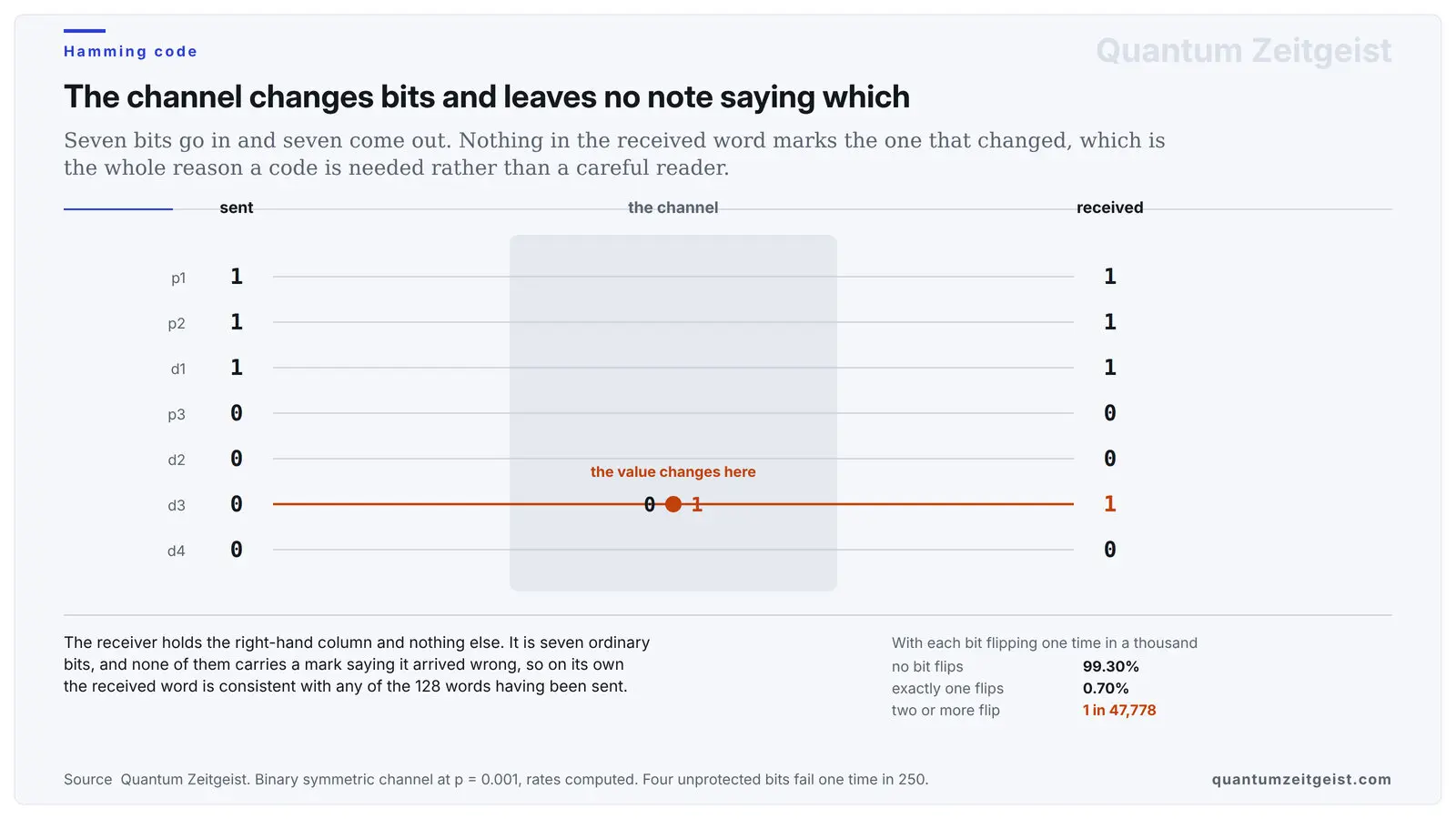
Start with what the channel does, because the code is an answer to it. A binary symmetric channel takes each bit and independently flips it with some small probability, so seven bits go in and seven come out with nothing marking which ones changed. The received word is seven ordinary bits, and on its own it is consistent with any of the 128 possible words having been sent.
The rates decide what is worth engineering for. With each bit flipping one time in a thousand, a seven-bit word arrives untouched about 99.3 per cent of the time, carries exactly one wrong bit about 0.7 per cent of the time, and carries two or more only about one time in 48,000. A scheme that repairs one error and notices two therefore covers nearly everything the channel actually does, and that is the trade Richard Hamming was making.
The classical Hamming code takes four data bits and adds three parity bits, producing a seven-bit block. That is written [7,4,3], meaning seven bits total, four of data, and a minimum distance of three between valid codewords.
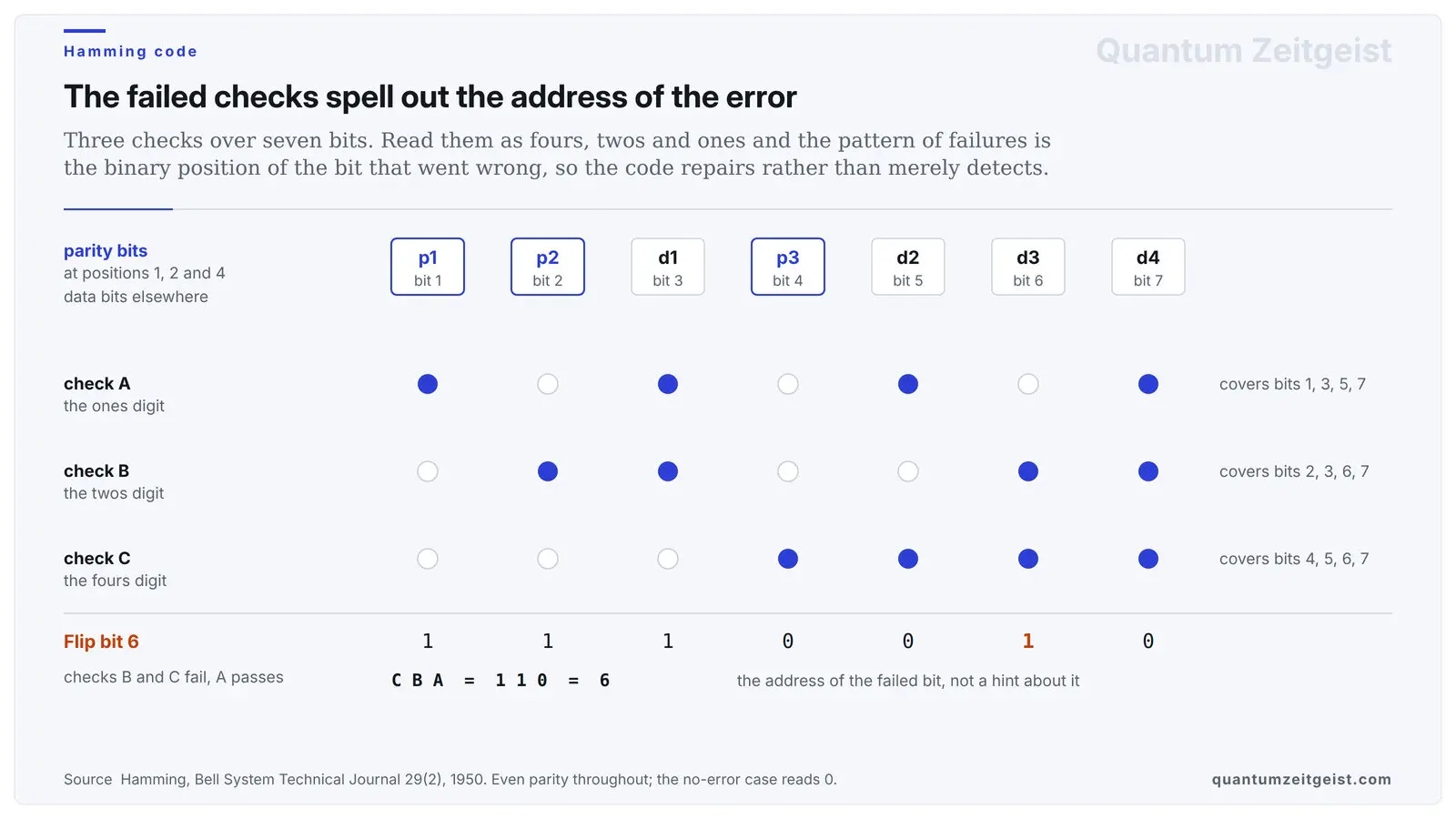
The grouping is easier to see than to state. Check A holds p1 together with d1, d2 and d4, check B holds p2 with d1, d3 and d4, and check C holds p3 with d2, d3 and d4, which puts d4 in all three because its position, seven, is 111 in binary. Drawn as three overlapping circles, each one has to come out even, and a single wrong bit turns exactly the circles that contain it odd.
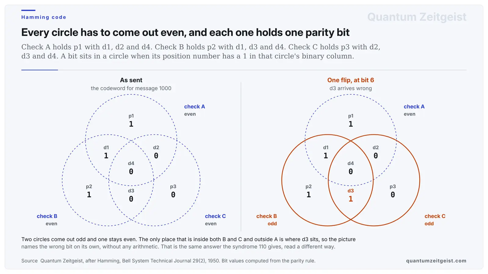
The elegance is in where the parity bits go. Each check covers a specific subset of positions, chosen so that position n is included in a check exactly when n has a one in the corresponding binary digit. Check A covers positions 1, 3, 5 and 7, check B covers 2, 3, 6 and 7, and check C covers 4, 5, 6 and 7.
Now flip a bit and see what happens. If bit 6 is corrupted, checks B and C fail while A passes, and reading the checks as C, B, A, that is as the fours, twos and ones digits, gives 110, which is six. The pattern of failures is not a clue to be interpreted. It is the address of the error, written in binary by the structure of the code itself.
Why parity was not enough
To see why Hamming’s code mattered, it helps to know what came before it. A single parity bit appends one bit recording whether the number of ones in a block is odd or even. If a bit flips, the count changes and the parity no longer matches, so the receiver knows something is wrong.
That is all it knows. A single parity bit cannot say which bit changed, and if two bits flip it reports no error at all, because the count returns to its original parity. Detection without location was the state of the art. Hamming’s 1950 paper begins from that family of detecting codes and moves to a single parity check on binary data, which is the step he then pushed further.
His insight was that several parity bits, each covering a carefully chosen overlapping subset of positions, together carry far more information than the same bits used independently. The overlaps are the whole point, since a given data bit participates in several checks, and the particular combination of checks it belongs to is what pins down its position when it fails.
Hamming distance
Richard Hamming defined the distance that carries his name as the number of positions where two strings differ, counted and nothing more. The strings 1110000 and 1110010 differ only at position six, so the distance between them is one, and that plain count is what turns error correction into a question about geometry.
The minimum distance of a code is the smallest distance between any two of its valid codewords, and for this one it is three. The pair worth checking first is 0000000 and 1110000, because a linear code always contains the all-zero word and 1110000 is one of its lightest non-zero codewords. If any two codewords in this code sit close together it is those two. Encoding the message 0000 gives 0000000 and encoding 1000 gives 1110000, and they differ in three places, at positions one, two and three.
Running all sixteen messages through the parity rule settles it. Seven of the resulting codewords carry exactly three ones and none carries fewer, and since the code is linear the difference between any two codewords is itself a codeword. That lightest codeword therefore fixes the smallest gap anywhere in the set, which is why the code is written [7,4,3] with the distance as its third number.
![All sixteen codewords of the [7,4] Hamming code, with the number of ones in each and the seven lightest highlighted](https://quantumzeitgeist.com/wp-content/smush-webp/hs_ham_distance.jpg.webp "Richard Hamming, The Man Who Made Computers Reliable")
Distance three is what pays for the correction. Every seven-bit string sits within one flip of at most one codeword, because two codewords would have to be closer than three apart for their one-flip neighbourhoods to touch. The decoder can therefore take any received string, find the nearest codeword and return it, with no ambiguity to resolve.
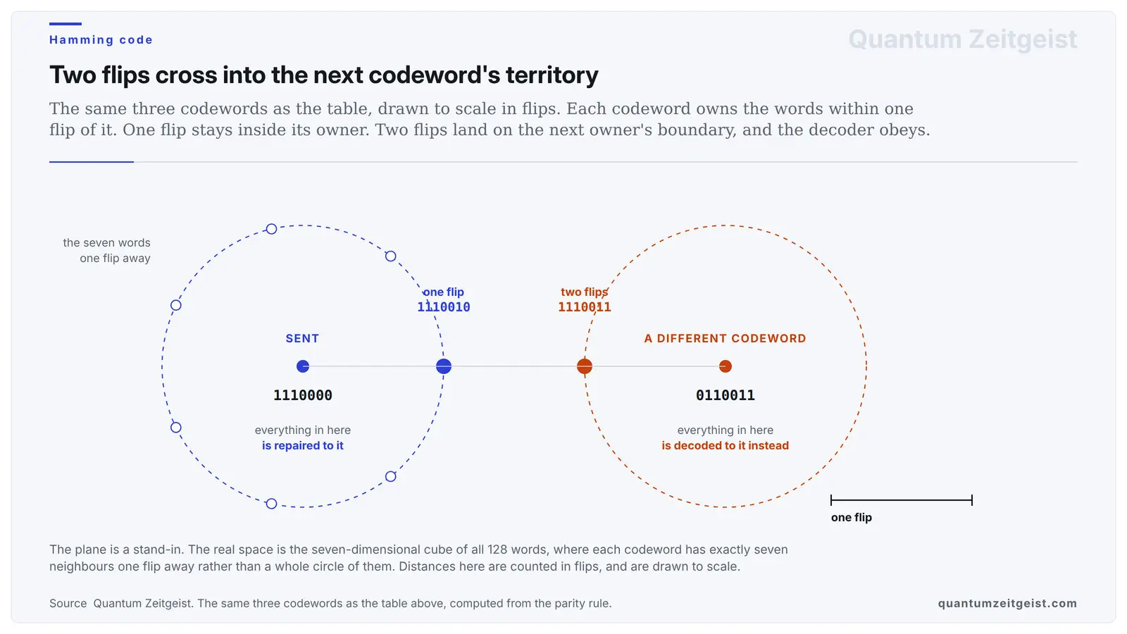
One error is repaired exactly. Flip bit six of 1110000 and the received string is 1110010, where checks B and C fail while A passes, so the syndrome reads 110, which is six in binary. Flipping bit six back recovers the message 1000, and nothing about the recovery is a guess.
Two errors are a different matter, and the failure is worth watching closely. Flip bits six and seven and the received string is 1110011, where only check A fails, so the syndrome reads 001 and addresses bit one. The decoder duly flips bit one and hands back 0110011, which is a perfectly valid codeword carrying the message 1011 rather than the 1000 that was sent. Every check passes on the way out, so nothing anywhere reports a problem, and two errors have produced a wrong answer rather than an error message.
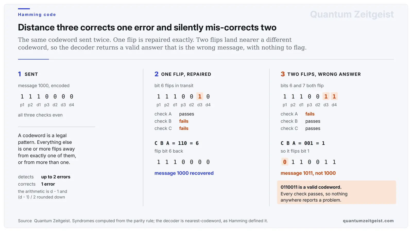
The general rule follows immediately. A code detects up to one error fewer than its distance, and corrects up to half of that number rounded down, so a distance of three detects two errors and corrects one. Richard Hamming set out that trade in the 1950 paper, and it is why quantum codes are written with three numbers such as [[7,1,3]], where the third is the closely analogous quantum distance, the smallest number of qubits an undetectable error must touch.
Shannon and Hamming, down the hall from each other
Two years before Hamming’s own paper appeared, Claude Shannon published the theorem establishing that reliable communication through a noisy channel is possible below a certain rate. The proof was non-constructive, showing that good codes must exist by arguing that a randomly chosen one is usually good, and offering no way to build a specific example.
The tidy story stops there, and the truth is better. Shannon’s 1948 paper does not merely fail to construct a code, it prints one, and the code it prints is Richard Hamming’s, credited to him by name in a section on efficient coding. The two men shared an office at Bell Labs for a time, and as Hamming put it, while Shannon was doing information theory he was doing coding theory. The existence proof and the explicit construction were not two years apart. They were the same building, the same corridor and, in 1948, the same paper.
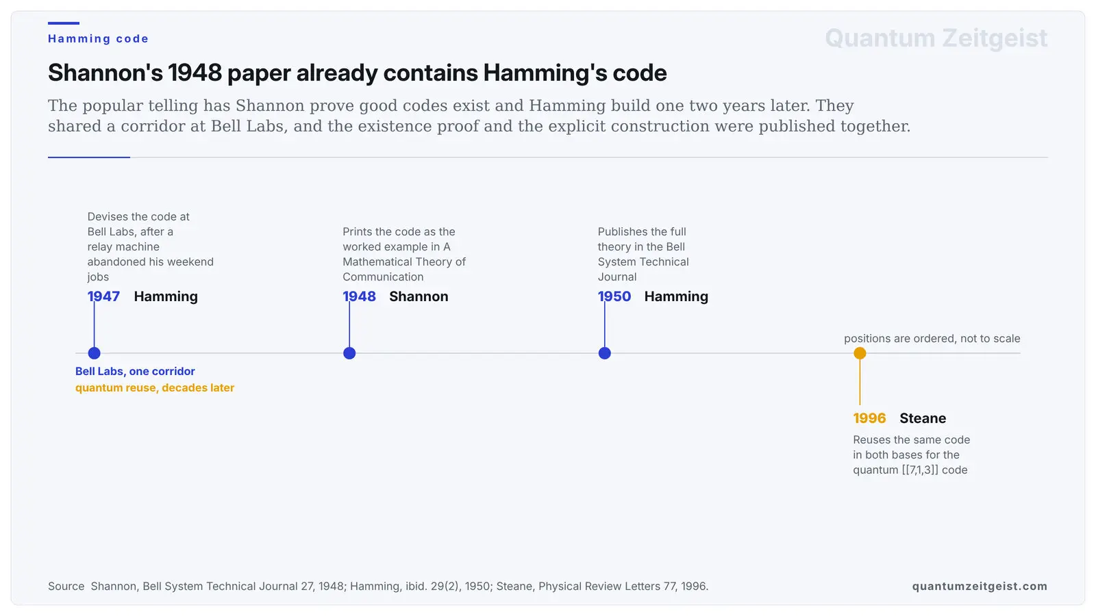
The two men were at Bell Labs at the same time, working on complementary halves of one problem. Shannon established what was possible and Hamming produced something you could implement, and the field has needed both kinds of result ever since.
The pattern repeated in quantum computing almost exactly. The early theoretical arguments established that quantum error correction was not forbidden, and the explicit codes followed, with Peter Shor’s nine-qubit construction in 1995 and Andrew Steane’s seven-qubit code in 1996.
The Hamming bound and perfect codes
Hamming also derived a limit on how efficient any such code can be. The reasoning is geometric, since each codeword needs a surrounding region of strings that decode back to it, and those regions cannot overlap.
Count the strings and you get an upper bound on how many codewords fit, now called the Hamming bound or the sphere-packing bound. A code achieving it exactly wastes nothing, and such codes are called perfect. Hamming codes form an infinite family of them, one for every number of parity bits, and Tietäväinen later proved that essentially the only perfect codes are the Hamming codes and the two Golay codes. The [7,4,3] is the smallest useful member, which is part of why it recurs so persistently.
The quantum version of this counting argument is the quantum Hamming bound, and it constrains how many logical qubits a code of a given size and distance can protect. The counting argument transfers to non-degenerate codes, of which the Steane code is one. Whether a degenerate code can beat the bound is still an open problem, which is a reminder that the quantum case is rarely quite as tidy as the classical one.
Why quantum error correction looked impossible
For some years after quantum computing was proposed, protecting quantum information looked unachievable. The objections were serious rather than technical, and each one seemed to rule the whole enterprise out.
Classical error correction depends on copying, and the no-cloning theorem forbids copying an unknown quantum state. It depends on measuring the received data to find the error, and measurement destroys superposition. Classical errors are also discrete, a bit is either flipped or not, whereas a qubit can be perturbed by any amount in a continuous space of possible errors.
Each of those turned out to be surmountable, and the resolutions are worth naming. Instead of copying, you spread one logical qubit across several physical ones. Instead of measuring the data, you measure relationships between qubits, which reveal whether an error occurred without revealing what the state is. And continuous errors, remarkably, collapse onto a discrete set when you make that measurement, so correcting bit flips and phase flips is sufficient to correct everything.
The Hamming code inside the Steane code
That last point is where Hamming’s work re-enters, because if only two kinds of error need correcting then two classical codes might handle them. This is the insight behind the CSS construction, named for Robert Calderbank, Peter Shor and Andrew Steane, and the Steane code is its most famous instance.
The Steane code encodes one logical qubit in seven physical qubits with distance three, written [[7,1,3]]. It uses the classical [7,4,3] Hamming code for both jobs at once, catching bit flips in the computational basis and phase flips in the conjugate basis, which is legal only because the Hamming code contains its own dual, the [7,3,4] simplex code. Hamming’s 1950 construction is not an analogy here, it is a component, used for exactly the job he designed it for.
The reason it fits is a property of the code Hamming had no reason to care about. The Hamming code contains its own dual, and that algebraic fact makes the bit-flip checks and the phase-flip checks compatible, so both can be measured simultaneously without interfering. A convenience of a 1950 telephone-engineering construction turned out to be the hinge on which quantum error correction swings.
The continuous error that becomes discrete
One step in quantum error correction is strange enough to deserve its own explanation, because it is the reason a finite classical code can protect against an infinite family of quantum errors. A classical bit fails in one way, by flipping. A qubit can be rotated by any angle, nudged a little or a lot, in a continuous space of possible disturbances.
It would seem to follow that you need infinitely many corrections, one for every possible rotation. You do not, and the reason is measurement. When the code’s parity-style checks are measured, the act of measuring forces the continuous error to collapse onto a discrete outcome, either a definite bit flip, a definite phase flip, both, or neither.
So the correction that follows only ever has to deal with those discrete cases, even though the error that occurred was continuous. A small over-rotation is not corrected as a small over-rotation. It is projected, by the measurement, into either no error or a full flip, and then handled as such. This is why counting bit flips and phase flips exhausts the problem, and it is what let Hamming’s discrete, classical logic survive the move to a continuous quantum world.
What came after the Hamming code
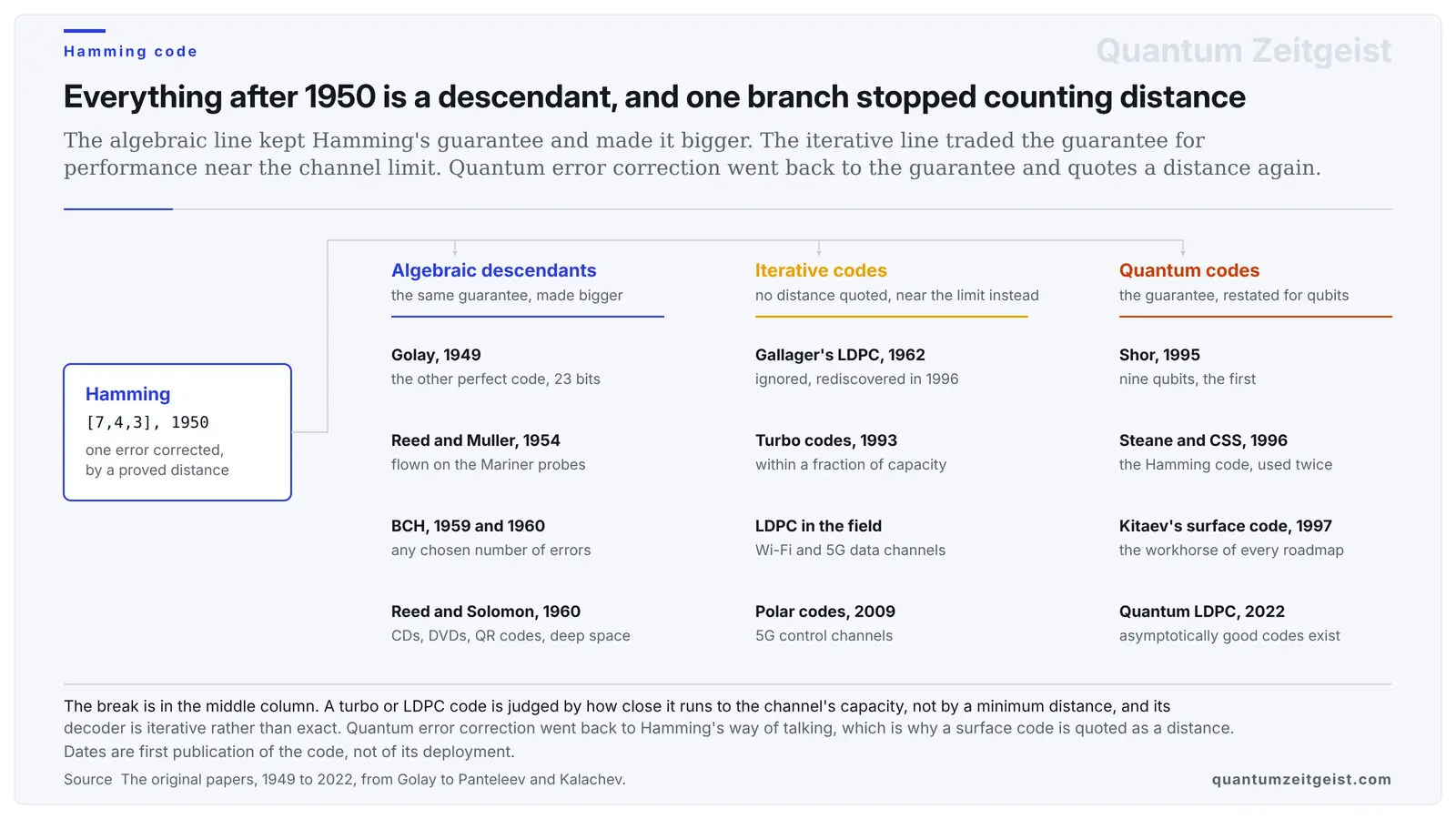
The 1950 construction turned out to be the first member of a family rather than a one-off. Marcel Golay had already published a perfect code of his own in 1949, and the algebraic line that followed kept the guarantee and made it larger, running through Reed and Muller in 1954, the BCH codes at the end of that decade, and Reed and Solomon in 1960. That last one is the code inside every compact disc, DVD and QR code, and it flew on deep space missions where asking for a retransmission takes hours.
The second branch broke with Hamming in a way worth understanding. Robert Gallager described low-density parity-check codes in 1962 and the idea was largely ignored for thirty years, until turbo codes arrived in 1993 and showed that iterative decoding could run within a fraction of a decibel of Shannon’s limit. Those codes are not judged by a minimum distance at all. They are judged by how close to capacity they run and how steeply their error rate falls, and their decoders are iterative rather than exact, so the clean promise that a distance-three code repairs one error has no counterpart in them.
That makes the quantum branch a deliberate return. Peter Shor’s nine-qubit code of 1995 and Steane’s seven-qubit code of 1996 brought the argument back to distance, and every serious fault-tolerant proposal since has been quoted the same way. A surface code at distance twenty-five is making exactly the claim the [7,4,3] code makes at distance three, that a stated number of simultaneous failures is survivable and the next one is not.
Where Hamming codes still run
The 1950 code is not a museum piece. Variants of it correct single-bit errors in computer memory, where the standard ECC arrangement in server RAM is a Hamming-style SECDED code, the construction extended with one more parity bit so it can also detect double errors.
Related schemes appear in flash storage, satellite links and any channel where retransmission is expensive or impossible. The technique is invisible precisely because it works, and a modern machine performs Hamming-style corrections continuously without reporting them.
| Concept | Hamming, 1950 | Quantum counterpart |
|---|---|---|
| Code parameters | [7,4,3], seven bits carrying four | [[7,1,3]], seven qubits carrying one |
| Distance | Minimum Hamming distance between codewords | Same definition, same role in the notation |
| Error location | Failed parity checks read as a binary address | Syndrome measurement, revealing the error not the state |
| Efficiency limit | The Hamming or sphere-packing bound | The quantum Hamming bound |
| What is protected | Bit flips | Bit flips and phase flips, needing two codes |
You and Your Research
In 1986 Hamming gave a talk at Bellcore that has circulated ever since, usually under the title You and Your Research. It asks why some scientists do significant work and others, with comparable ability and resources, do not.
His answer is uncomfortable and largely about deliberate choice. He argues that most researchers never sit down and identify the important problems in their field, that working with an open door costs short-term productivity and pays back enormously in relevance, and that courage is a research skill because important problems look intractable until someone attacks one.
The talk is worth reading in full by anyone choosing research directions, and quantum computing is a field where the question bites. There is a great deal of work that is publishable and a much smaller amount that changes what is possible, and telling them apart in advance is exactly the skill Hamming was describing.
What Hamming teaches about reading claims
There is a habit of mind in Hamming’s work that transfers usefully to assessing quantum computing claims, and it is worth stating on its own. He was relentlessly concrete. He did not argue that errors could in principle be corrected, he built the thing that corrected them and showed exactly how many bits it cost.
Applied to quantum error correction, that habit turns vague reassurance into specific questions. A code does not simply protect a qubit, it protects one logical qubit using a stated number of physical ones, at a stated distance, correcting a stated number of errors. When someone says a machine is fault tolerant, the concrete follow-up is which code, at what distance, with what physical error rate, and how many physical qubits per logical one.
Those numbers are where the real state of the field lives. A distance-three code like Steane’s corrects one error, which is a demonstration rather than a useful computer, and reaching the millions of physical qubits that a useful machine needs is the actual engineering problem. Hamming’s insistence on counting is the fastest route to seeing that clearly, and it is the same discipline that runs through the rest of this material.
What he left behind
The name of Richard Hamming is attached to more objects than most mathematicians manage, including a distance, a bound, a window function in signal processing and a family of codes. The common thread is that each began as a practical annoyance rather than an abstract question.
The deeper contribution is the idea that reliability can be engineered into information itself rather than into the hardware carrying it. Before 1950 the way to reduce errors was better components and more power. After 1950 you could add structured redundancy and get correctness out of unreliable parts, which is the principle every fault-tolerant quantum architecture now depends on.
That is a striking inheritance for work that started with a lost weekend of computing time. Hamming decided the machine ought to do better, and the principle he found reaches all the way into the hardware being built today.
Frequently asked questions
Who was Richard Hamming?
Richard Hamming was an American mathematician, born in 1915 and died in 1998, who invented the first practical error-correcting codes. He worked on the Manhattan Project at Los Alamos, spent thirty years at Bell Labs, and received the Turing Award in 1968.
What is a Hamming code?
It is an error-correcting code that adds parity bits to a block of data so that a single corrupted bit can be located and repaired. The classical version takes four data bits and adds three parity bits, and the pattern of failed parity checks reads directly as the binary position of the error.
What is Hamming distance?
It is the number of positions at which two strings differ. Error-correcting codes work by keeping valid codewords a minimum distance apart, so that a corrupted word is still closer to its original than to any other valid codeword.
How is the Hamming code related to the Steane code?
The classical [7,4,3] Hamming code is a component of the quantum [[7,1,3]] Steane code. The Steane code uses it for both error types at once, correcting bit flips in one basis and phase flips in the other, an arrangement called the CSS construction. Hamming’s code is not an analogy in that setting, it is literally part of the machinery.
Did Hamming work with Claude Shannon?
They were both at Bell Labs in the same period and worked on complementary halves of the same problem. Shannon proved in 1948 that reliable communication through noise is possible without constructing a code, and Hamming published an explicit code in 1950.
Are Hamming codes still used?
Yes. Variants correct single-bit errors in computer memory, with the common ECC arrangement in server RAM being a Hamming code with an extra parity bit added so it can also detect double errors. Related schemes appear in storage and communication systems generally.
What is You and Your Research?
It is a talk Richard Hamming gave in 1986 on why some scientists do important work and others do not. He argues it is largely a matter of deliberate choice, including choosing important problems, keeping your door open to colleagues, and having the courage to attack problems that look intractable.
What is the Hamming bound?
It is a limit on how many codewords a code can contain given its length and the number of errors it must correct, derived by counting how many strings must decode to each codeword. Codes that meet it exactly are called perfect, and the [7,4,3] code is one. A quantum version constrains quantum codes the same way.




See today’s quantum computing news on Quantum Zeitgeist for the latest breakthroughs in qubits, hardware, algorithms, and industry deals.