

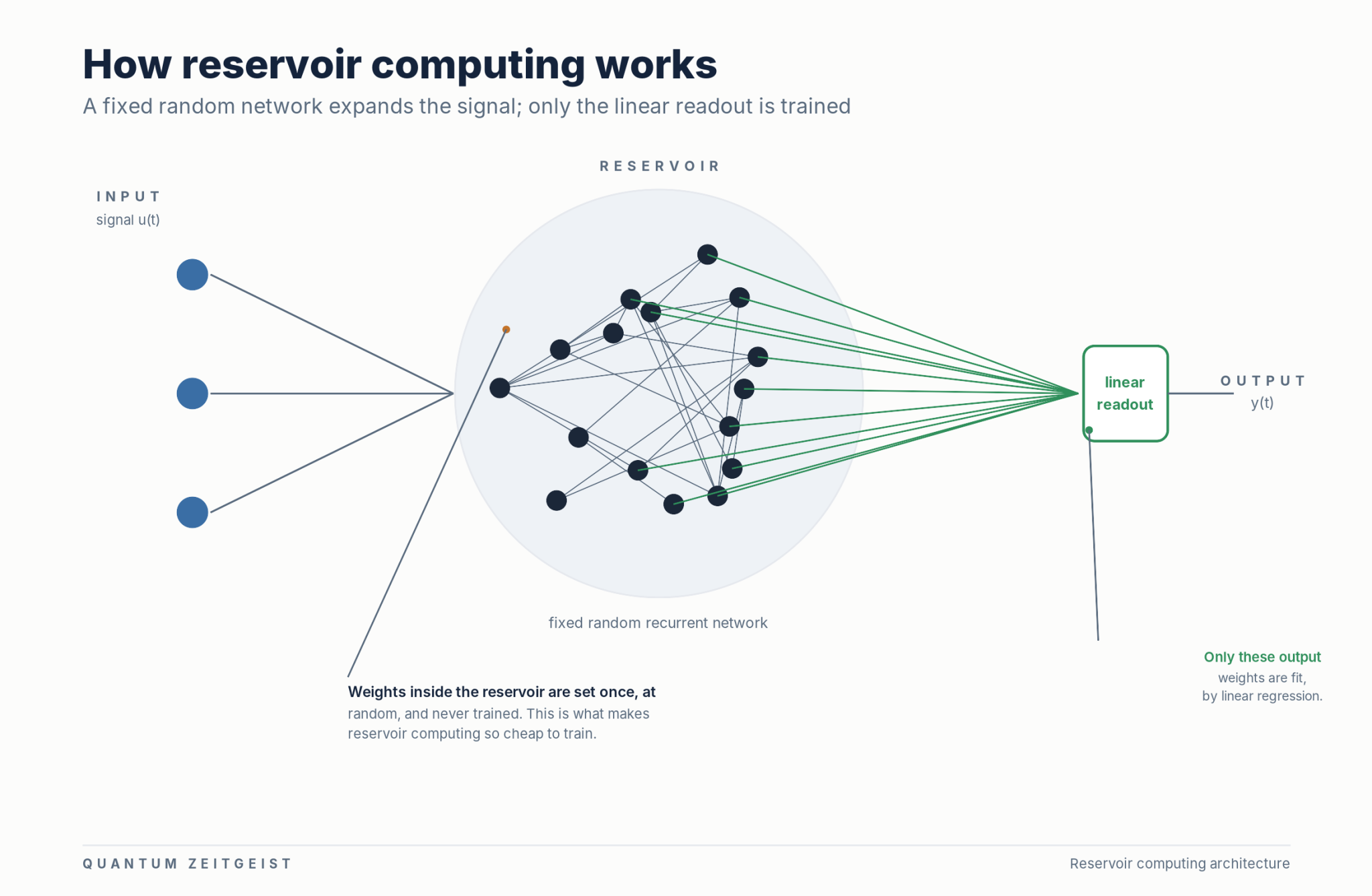
Reservoir computing is a way to build a machine that understands signals that change over time, without paying the heavy training bill of a normal recurrent neural network. The trick is simple to state. You take a large, fixed, randomly wired network, feed your signal into it, and let its internal activity swirl into a rich pattern. Only a small output layer, called the readout, is ever trained. Everything inside the network stays frozen.
That single idea, keeping the recurrent core fixed and training only a linear readout, is what makes reservoir computing fast, cheap, and easy to run on unusual hardware. It also travels well into the quantum world, where a handful of qubits can stand in for the reservoir and open up a feature space far larger than the physical device. This guide walks through the core idea, the two classic families, the physical and quantum versions, and where the method is actually used today.
The core trick. Reservoir computing freezes a large random recurrent network and trains only a simple linear readout, so learning becomes a single regression step.
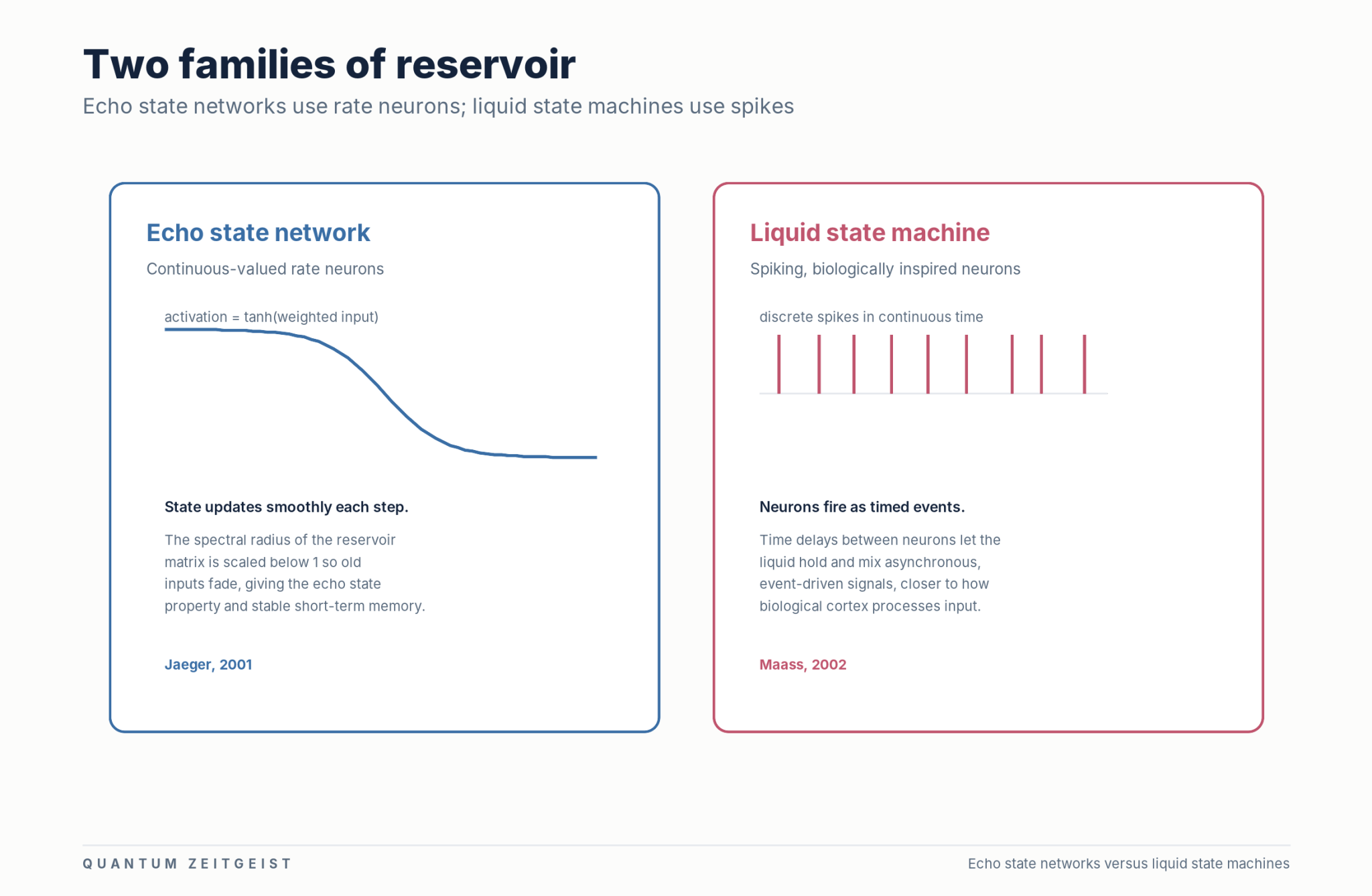
Two founding families. Echo state networks use continuous rate neurons, while liquid state machines use spiking neurons; both were proposed independently around 2001.
The echo state property. A working reservoir must forget its distant past, so its response depends on recent input rather than on where it happened to start.
Reservoirs can be physical. Light in a photonic chip, a spintronic oscillator, a memristor, or even a bucket of water can serve as the reservoir.
Quantum reservoirs go further. A few qubits span an exponentially large space, so a quantum reservoir can supply many features from very little hardware.
Best at time. The method shines on chaotic forecasting, temporal signal processing, and low-power edge learning, where fast training and low latency matter most.
What reservoir computing actually is
A recurrent neural network processes a sequence one step at a time, and it keeps a hidden state that carries information forward. Training a full recurrent network means adjusting every weight by backpropagation through time, which is slow and often unstable. Reservoir computing sidesteps that whole problem. It keeps the recurrent part fixed and trains only the layer that reads the state out.
The fixed recurrent part is the reservoir. It is usually a sparse network of nonlinear nodes with random connection weights, and those weights never change once they are set. When a signal enters, the reservoir reacts, and its many internal activations become a high-dimensional picture of the recent input. Patterns that were tangled together in the raw signal often become easy to separate in that larger space.
The readout is the only trained part. It is a plain linear map from the reservoir state to the output you want, and it is fit with ordinary least squares or ridge regression. Because the mapping is linear and the reservoir does the hard nonlinear work, one pass over the training data is usually enough. Our earlier explainer on reservoir computing and efficient neural networks covers the same idea from an applications angle.
It helps to think of the reservoir as a nonlinear echo chamber. Each new input excites it, the excitation lingers and mixes with earlier excitations, and the readout learns to pick out the combinations that matter. The reservoir supplies memory and nonlinearity for free, and the training reduces to fitting a straight line through those features.
There is a useful way to see why this works at all. A linear model cannot separate patterns that are tangled together, but the same patterns often pull apart once they are lifted into a much larger space. The reservoir performs that lift, projecting a short slice of the input into hundreds of nonlinear coordinates. This is the same intuition behind kernel methods, and it is why a linear readout on top of a rich reservoir can solve problems that look nonlinear from the outside.
Echo state networks and liquid state machines
Two research lines arrived at this idea at almost the same time, around 2001, and both are still in active use. Herbert Jaeger, then at the German National Research Center for Information Technology, described echo state networks in a 2001 technical report and later built his group at Jacobs University Bremen. Wolfgang Maass and colleagues, working from computational neuroscience, introduced liquid state machines in the same period. The umbrella term reservoir computing came later, once people saw the two were the same recipe.
The name was popularised through the second half of the 2000s as researchers unified the two threads, with a widely cited 2009 review by Mantas Lukoševičius and Herbert Jaeger gathering the methods under one banner. The roots run deeper still, into 1990s computational neuroscience models of how cortical circuits turn time-varying input into separable activity. What Jaeger and Maass added was the practical realisation that the recurrent part could stay fixed, which is the move that made the approach cheap and general.
Echo state networks
An echo state network uses continuous-valued neurons whose activation is a smooth function, typically a hyperbolic tangent of the weighted input. The reservoir weights are drawn at random and then rescaled so the network sits in a useful dynamical regime. This is the version most people reach for first, because it is a handful of matrix operations and needs no special hardware to run.
Tuning an echo state network is mostly about a few global numbers rather than millions of weights. The spectral radius sets how long memory lasts, the input scaling sets how hard the signal drives the reservoir, and the sparsity sets how densely the nodes connect. Those knobs are far easier to search than a full weight matrix, which is a large part of the appeal.
Liquid state machines
A liquid state machine takes a more biological route. Instead of smooth rate neurons it uses spiking neurons that fire as discrete events in continuous time, with time delays on the connections between them. That structure lets the liquid hold and mix asynchronous, event-driven signals in a way that mirrors cortical processing.
The name comes from an image of dropping a stone into liquid and reading the ripples. Any perturbation leaves a fading trace, and a readout trained on the current ripple pattern can recover what happened recently. Liquid state machines are a natural fit for neuromorphic chips that already speak in spikes, which is why they appear often in low-power hardware research.
The echo state property and fading memory
A reservoir is only useful if its state reflects the input rather than the accident of where it started. That requirement has a name, the echo state property. It says that after enough time the reservoir forgets its initial condition, so any two runs on the same recent input settle into the same state. Without it, the readout would be learning from noise about the starting point instead of signal about the data.
The spectral radius of the reservoir weight matrix is the main lever here. It is the largest magnitude among the eigenvalues of that matrix, and it controls how strongly past activity feeds back. Push it too low and the reservoir forgets almost instantly, erasing the memory you need. Push it too high and the dynamics turn chaotic, so tiny differences blow up and the response becomes unpredictable.
The usual rule of thumb is to scale the reservoir so the spectral radius sits a little below one, which keeps memory long but stable. The sweet spot depends on the task, since a signal with long dependencies needs more memory than a fast reactive one. This balance between memory and stability is the single most important thing to get right in a classical reservoir.
The story becomes richer in the quantum setting, where researchers have shown that useful computation can happen even when the strict echo state property is bent. One study on a quantum reservoir that exploits memory and violates the echo state property found that controlled memory effects can help rather than hurt, and separate work extended the property to non-stationary quantum systems where the reservoir itself drifts over time.
Why reservoir computing is so cheap to train
The cost of training a normal recurrent network grows with the number of weights and the length of the sequences, because gradients have to flow backward through every step. That process can vanish, explode, or simply take a long time. Reservoir computing removes it entirely for the recurrent part, since those weights are fixed and no gradient ever touches them.
Once you run your training signal through the reservoir, you collect its states into a matrix and solve one linear system for the readout. That is a convex problem with a closed-form answer, so there is no risk of getting stuck in a bad local minimum and no long schedule of gradient steps. The same fixed reservoir can also be reused across different tasks, since only the readout needs to be refit.
This economy is why the approach keeps drawing interest for real-time and resource-limited work. Researchers have pushed it further by cutting the time complexity of the readout stage, as in work that reduced the time complexity of a quantum reservoir while improving performance, and by pairing reservoirs with generative models to raise accuracy using a generative adversarial network. The theme across all of it is the same, do the expensive nonlinear work once and keep learning linear.
Benchmarks and memory capacity
Reservoirs are usually judged on a small set of standard tasks. The NARMA benchmark asks the system to reproduce a nonlinear autoregressive sequence, while the Mackey-Glass and Lorenz systems test forecasting of chaotic signals. These tasks reward exactly the two things a good reservoir provides, memory of the recent past and a nonlinear mixing of it.
Memory itself can be measured. The linear memory capacity of a reservoir counts how many past inputs the readout can reconstruct, and for a network of a given size that capacity is bounded by the number of nodes. There is a tension to manage, since squeezing more nonlinearity out of a reservoir tends to shorten its memory. Choosing the spectral radius and input scaling is really a way of setting where you sit on that trade-off.
Physical reservoirs, from photonics to water
Nothing in the recipe says the reservoir has to be simulated on a computer. Any physical system that is nonlinear, has some memory, and can be driven by an input and observed at the output can serve as the reservoir. This is called physical reservoir computing, and it turns the fixed random network from a piece of software into a piece of matter.
Photonic reservoirs
Light is a natural medium for this, because it is fast, parallel, and nonlinear at the right power levels. A common design uses a single nonlinear optical node with a delay loop, which unfolds in time into a virtual network of nodes. Integrated versions put the whole reservoir on a chip, as in work where a silicon microring resonator used thermal nonlinearity to classify digits.
Spintronic and electronic reservoirs
Magnetic devices offer another route. In 2017 a team showed that a single nanoscale spin-torque oscillator, a magnetic tunnel junction smaller than a micron, could recognise spoken digits at accuracy close to standard neural networks, using its own nonlinear oscillation as the reservoir. Electronic reservoirs work too, and a ferroelectric transistor has been used to speed reservoir computing with dual memory operation.
Memristors and unconventional media
Memristors are resistors whose state depends on their history, which makes them a compact source of memory and nonlinearity. Groups have built small reservoirs from dynamic memristor arrays, and more exotic work has explored dynamic reservoirs and DNA-based memristors for temporal processing. The idea reaches its playful extreme in a 2003 demonstration where the reservoir was literally a bucket of water, with ripples on the surface doing the nonlinear mixing before a simple readout solved a pattern task.
The trade-offs differ from software reservoirs. A physical medium processes the signal at the speed of its own physics, which can be far faster than a digital step, and it spends little energy doing so. The cost is that real devices drift, add noise, and cannot be inspected node by node, so the readout has to be robust to a reservoir that is never quite the same twice. In practice this suits streaming sensor tasks better than problems that demand exact repeatability.
Because the hardware itself supplies the dynamics, physical reservoirs can be very fast and very low power. That mix of properties has drawn attention from applied fields, and reservoir computing has been funded for defence and security sensing tasks where low latency on a compact device is worth a great deal.
Reservoir computing and neuromorphic chips
Liquid state machines and physical reservoirs share a home with neuromorphic hardware, the chips that mimic how neurons compute rather than how a processor does. Devices such as Intel Loihi and IBM TrueNorth use spiking neurons and event-driven communication, so a spiking reservoir maps onto them with little translation. The pairing is attractive because both sides aim at the same goal, useful computation at very low energy.
On this kind of chip the reservoir can run continuously while only the readout is retrained as conditions change, which fits robots and sensors that must adapt in place. Work on spiking networks on Loihi hardware for autonomous robot control shows the style, a fixed recurrent substrate with a light, adaptable output. Reservoir computing gives that substrate a principled reason to stay fixed, which is why the two fields keep meeting.
Quantum reservoir computing explained
Quantum reservoir computing replaces the random network with a quantum system. You encode your classical input into the state of a few qubits, let that state evolve under a fixed quantum interaction, and then measure a set of observables to read out features. Just as in the classical case, the quantum evolution is not trained; only the linear readout on the measured features is fit.
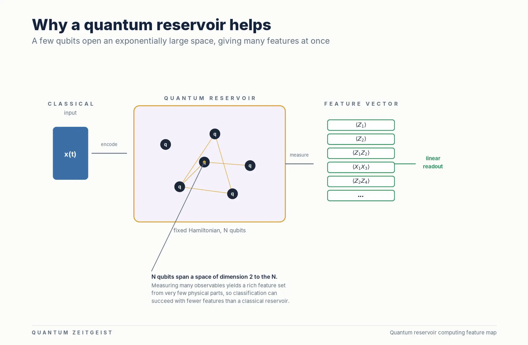
The reason this is interesting is a matter of size. A system of a few qubits lives in a space whose dimension grows as two to the power of the number of qubits, so even a small device offers an enormous internal space to work in. Measuring many observables of that state, single-qubit and correlated ones, gives a long feature vector from very little hardware. The idea was set out in a foundational 2017 paper by Keisuke Fujii and Kohei Nakajima, which showed that disordered quantum dynamics could serve as a machine-learning resource (the founding quantum reservoir computing paper).
That efficiency shows up directly in results. QZ has covered a quantum reservoir that achieves classification with fewer features than a classical model needs, and separate work in which a quantum reservoir learns from data without any training of the reservoir itself. The appeal is not raw speed but representational richness, a lot of useful features for a small physical footprint.
Measurement plays a subtle role that has no classical analogue. Reading out a quantum state disturbs it, so a quantum reservoir has to balance extracting features against preserving the dynamics that carry memory. Weak measurement, repeated preparation, and a small amount of engineered dissipation are common ways to keep the reservoir both informative and stable. On the noisy hardware available today, that noise is not always the enemy, since a controlled amount of it can wash out the initial state and supply the fading memory the method needs.
Quantum reservoirs also lean on quantum effects that have no classical counterpart. One study found that a reservoir can leverage correlations that go beyond what classical systems allow, and QZ has reported broader introductions to quantum reservoir computing for machine learning and a new quantum approach to the same problem. For a wider view of how learning meets quantum hardware, our pillar on quantum machine learning sets the context.
What quantum reservoir research is probing now
The quantum version is young, and much of the recent work is about understanding what these reservoirs can and cannot do. A few themes stand out, and QZ has followed most of them as the papers appeared. They give a good sense of where the method is being pushed.
Rydberg-atom reservoirs
Neutral atoms excited to high Rydberg states interact strongly and can be arranged in flexible patterns, which makes them a promising reservoir medium. Researchers have shown adversarial robustness and spatiotemporal pattern extraction with a Rydberg reservoir. The strong interactions give the reservoir a naturally rich response to input, which is exactly what a good feature map needs.
Photonic quantum reservoirs
Photons can carry the quantum reservoir as well as the classical one. Work on photon-number-resolving quantum reservoirs uses the statistics of detected photons as the feature set, aiming at high-speed processing. This line connects quantum reservoir computing to the wider push for optical machine learning hardware.
Detecting structure without labels
Quantum reservoirs are not limited to supervised tasks. One striking result used a reservoir for unsupervised detection of topological phase transitions without complex measurements, letting the physics of the reservoir flag where a material changes phase. Other work has shown that stable reservoirs can boost data processing, and QZ has covered quantum reservoirs that classify demanding engineering data.
Quantum reservoirs on real hardware
Most quantum reservoir results until recently lived in simulation, but the method has now run on real quantum processors at a meaningful scale. In 2024 a team from QuEra Computing, working with collaborators at Harvard and the University of Colorado, implemented quantum reservoir learning on QuEra’s Aquila machine, a neutral-atom analog processor. They encoded classical data into the atoms and read out local observables after a fixed evolution, using as many as 108 atoms in a single learning task. That run stands as one of the largest quantum machine-learning demonstrations reported so far.
The Aquila work fits the reservoir recipe well because an analog machine evolves its whole register under one programmable Hamiltonian rather than a trained gate sequence. The atoms supply the nonlinear mixing, and only the classical readout is fit, exactly as in a classical reservoir. The team reported competitive accuracy on binary and multi-class classification as well as time-series prediction, which are the standard reservoir tasks moved onto quantum hardware.
Superconducting devices have carried the idea too. In 2025 Carles, Dudas, Grollier, Markovic and colleagues built a quantum reservoir from a single transmon qubit coupled to a readout resonator, a circuit quantum electrodynamics setup, and classified data using many nonlinear features drawn from that one small system. IBM Research has separately reported reservoir and extreme-learning experiments on its utility-scale superconducting processors, running on more than a hundred qubits. The same pattern holds across platforms, a fixed physical evolution and a light trained readout.
These demonstrations come with a caveat that is easy to miss. A system of n qubits does span a space of dimension two to the n, but you cannot read out that many independent features, because every observable has to be estimated from a finite number of measurement shots. The statistical error on an expectation value falls only as one over the square root of the shot count, so resolving many features to good precision costs many repetitions, and hardware noise erodes them further. The usable feature count therefore scales with your measurement budget and device fidelity, not with the raw size of the state space.
The practical lesson is that scale on paper and scale in practice are different things for quantum reservoirs. The Aquila and transmon experiments matter because they test the method against real noise, finite sampling, and imperfect control rather than idealised dynamics. For now the honest claim is representational richness from a small device, not an exponential free lunch, and the open question is whether a quantum reservoir can beat a well-tuned classical one on a task that counts. That comparison, run fairly on hardware, is where the field is heading.
What reservoir computing is used for
Reservoir computing is at its best when the data has a time axis, since memory and nonlinearity are exactly what temporal problems need. The applications below are the ones where it competes with or beats heavier models, and they share a common shape, streams of data that must be processed quickly and often on modest hardware.
Chaotic time-series forecasting
Predicting chaotic systems is a signature strength. In 2018 Edward Ott’s group at the University of Maryland, with Jaideep Pathak as first author, showed that a reservoir could forecast the evolution of a spatiotemporally chaotic system from data alone, with no model of the underlying equations, staying accurate for several Lyapunov times. That result made reservoir computing a serious tool for weather-like and turbulence-like prediction, where short-term forecasts are valuable and full models are expensive.
The reason chaos suits the method is that chaotic systems are deterministic but sensitive, so short-horizon prediction is possible while long-horizon prediction is not. A reservoir can learn the local rule that advances the state a step, then be run in a loop to roll that rule forward. Because only the readout is fit, the whole predictor can be trained from a single trajectory, which is a real advantage when data is scarce.
Temporal signal processing
Speech recognition, channel equalisation in communications, and biomedical signals such as electroencephalogram traces all fit the reservoir mould. The reservoir turns a raw waveform into features that a linear readout can classify, which suits streaming data that arrives one sample at a time. Physical reservoirs are attractive here because they can process the signal in the same medium that carries it.
These tasks also explain why the method rewards careful input handling. A signal that is scaled well and fed in at the right rate drives the reservoir into its most expressive regime, while a poorly scaled one either barely moves it or saturates it. In communications, the same setup that equalises a distorted channel can be retrained in seconds when conditions shift, which is exactly the kind of fast adaptation that a fully trained network struggles to match.
Low-power edge learning
Because only a small readout is trained, reservoir computing fits devices that cannot afford to run backpropagation. A sensor node can carry a fixed physical reservoir and update just its output weights, which keeps power and memory low. This edge angle overlaps with neuromorphic engineering and with efforts to run learning on the same silicon that does other work, as in a silicon chip that performs both quantum and standard machine learning tasks.
The efficiency case can be dramatic. In one adjacent industry example, a quantum system trained in days rather than months rivalled a deep-learning baseline; it was not a reservoir computer, but it chased the same promise of strong results from a light training budget. For readers who want the hardware landscape behind these efforts, our guide to the top quantum hardware companies and to silicon spin quantum computing companies map out who is building the devices.
Strengths and limits of the method
The strengths are easy to summarise. Training is fast and stable, the same reservoir can be reused, the method handles noise gracefully, and it maps neatly onto physical and quantum hardware. For streaming and real-time work, that combination is hard to beat with a fully trained network.
The limits are just as real. A fixed random reservoir is not tuned to your task, so it can miss long-range structure that a fully trained network would capture. Designing a good reservoir still involves searching over the spectral radius, sparsity, and input scaling, and a poor choice can quietly cap performance. On the hardest problems, a deep model with millions of trained weights will usually win on raw accuracy.
Some of these limits are being chipped away. A 2021 method called next-generation reservoir computing drops the random network and instead builds the feature vector directly from nonlinear functions of recent inputs, which cuts the data and tuning a traditional reservoir needs. Approaches like this keep the cheap linear readout while removing the awkward search for a good random reservoir, and they show the field is still moving.
The table below sums up how reservoir computing sits against a fully trained recurrent network. The right choice depends on whether you value cheap, fast, hardware-friendly training or maximum accuracy on a complex task.
| Aspect | Reservoir computing | Fully trained RNN |
|---|---|---|
| What is trained | Linear readout only | All weights |
| Training cost | One regression, very low | Backpropagation through time, high |
| Stability of training | Convex, no local minima | Can vanish or explode |
| Hardware fit | Runs on photonic, spintronic, quantum media | Mostly digital accelerators |
| Peak accuracy | Strong on temporal tasks | Higher on the hardest problems |
| Main tuning knobs | Spectral radius, sparsity, input scaling | Architecture plus every weight |
Reservoir computing next to transformers and state-space models
Reservoir computing is not the only way to model sequences, and it helps to place it beside the architectures that now dominate. A transformer, introduced by Vaswani and colleagues in 2017, drops recurrence entirely and lets every position attend to every other through trained attention weights. All of its parameters are learned by gradient descent, its cost grows with the square of the sequence length, and it needs large data and compute to do well. Reservoir computing is almost its mirror image, a fixed recurrent core with a single trained linear readout.
State-space models sit between the two. The S4 model of Gu, Goel and Re in 2022, and the later Mamba model of Gu and Dao in 2023, use a linear recurrence much like an echo state network, but they train the recurrence itself rather than freezing it. Mamba makes its state updates depend on the input, which lets it choose what to remember, and both models handle long sequences at sub-quadratic cost. In effect they kept the cheap linear-recurrence backbone that reservoirs rely on and made it learnable.
Seen this way, the difference is what you are willing to train. Reservoir computing trains nothing in the recurrence and pays almost nothing to learn, while state-space models train the recurrence with gradients and pay more for a higher accuracy ceiling. Transformers train everything and buy the most expressive model at the highest cost. The three form a rough ladder from cheapest and most constrained to most powerful and most demanding.
That framing tells you when to reach for each. Reservoir computing wins where the training budget is tiny, the latency must be low, and the hardware is small or physical, such as an edge sensor, a photonic chip, or a few qubits, and it does well on chaotic forecasting from a single trajectory. It loses where data and compute are plentiful and the task rewards content-based selection over long contexts, which is the home ground of transformers and, increasingly, of state-space models. The right choice follows the budget more than the fashion.
How to build a reservoir computer
A first echo state network is short to write, and the steps make the ideas above concrete. The recipe is the same whether you run it in software or on physical hardware, only the reservoir changes. Working through it once removes most of the mystery.
Start by creating the reservoir. Fill a square weight matrix with random values, keep only a small fraction of them so the network is sparse, and rescale the matrix so its spectral radius sits a little below one. Add a random input matrix that injects your signal into the reservoir. These matrices are fixed for good and never trained.
Next, run your training signal through the reservoir step by step, applying the nonlinear activation at each step, and record the reservoir state every time. Stack those states into a matrix of features. Then fit the readout by solving a single ridge regression from the state matrix to your target outputs, which gives the output weights in one shot.
To use the trained system, drive the reservoir with new input, collect its state, and apply the readout to get a prediction. For forecasting, feed the output back in as the next input so the system runs on its own. From there you can swap the software reservoir for a physical one, or for a quantum reservoir, and the training stage barely changes.
Two practical details make the difference between a toy and a working model. Discard the first stretch of reservoir states, the washout, so the readout only sees states that have forgotten the arbitrary starting point. Use ridge regression rather than plain least squares, since the small penalty keeps the output weights from chasing noise and greatly improves how the model behaves on unseen data. Beyond those, the main effort is a modest search over the spectral radius and input scaling to match the memory your task demands.
Frequently asked questions
What is reservoir computing in simple terms
Reservoir computing is a machine-learning method that processes signals over time using a large fixed random network, called the reservoir, and trains only a small linear readout on top. The reservoir supplies memory and nonlinearity, so learning reduces to a single regression step.
How is reservoir computing different from a normal neural network
A normal recurrent network trains every weight by backpropagation through time, which is slow and unstable. Reservoir computing keeps the recurrent weights fixed and random and trains only the output layer, which makes training far cheaper and more stable.
What is the echo state property
The echo state property says the reservoir must forget its starting condition over time, so its state depends on recent input rather than on where it began. It is usually enforced by scaling the reservoir so its spectral radius sits a little below one.
What is the difference between echo state networks and liquid state machines
Echo state networks use continuous-valued rate neurons with smooth activations, while liquid state machines use spiking neurons and time delays. Both freeze the reservoir and train only a readout, but liquid state machines fit spiking neuromorphic hardware more naturally.
What is quantum reservoir computing
Quantum reservoir computing uses a quantum system as the reservoir. Classical input is encoded into a few qubits, a fixed quantum interaction mixes the state, and measured observables become the features for a linear readout, giving many features from little hardware.
Can a reservoir be a physical device
Yes. Any nonlinear system with memory can serve as a reservoir, including photonic chips, spintronic oscillators, memristors, and even ripples on water. This is called physical reservoir computing and can be very fast and low power.
What is reservoir computing good at
It is strongest on temporal tasks such as chaotic time-series forecasting, speech and signal processing, and low-power edge learning. Fast training and low latency are its main advantages over heavier models.
What are the main limits of reservoir computing
Because the reservoir is fixed and random rather than tuned to the task, it can miss long-range structure, and designing a good reservoir still needs a search over its parameters. On the hardest problems a fully trained deep model usually reaches higher accuracy.




See today’s quantum computing news on Quantum Zeitgeist for the latest breakthroughs in qubits, hardware, algorithms, and industry deals.