
1. Quantum decoherence is entanglement with the environment. A qubit in superposition becomes entangled with environmental degrees of freedom (air molecules, thermal radiation, magnetic-field fluctuations); tracing out the environment leaves the qubit in a classical mixture rather than a clean superposition.
2. T1 is energy relaxation; T2 is dephasing. T1 is the timescale over which an excited qubit |1⟩ decays to |0⟩; T2 is the timescale over which the relative phase between α|0⟩ and β|1⟩ randomises. The relationship 1/T2 = 1/(2T1) + 1/Tφ (where Tφ is the pure dephasing time) ties the two together.
3. The density matrix replaces the state vector. When a quantum system loses coherence, the state is no longer a single vector |ψ⟩ in Hilbert space but a probability mixture described by a density matrix ρ; off-diagonal elements (coherences) decay as decoherence progresses.
4. The Lindblad master equation is the standard tool. The Lindblad equation describes the time evolution of an open quantum system’s density matrix as a sum of unitary evolution plus dissipative terms; it is the canonical mathematical machinery for modelling quantum decoherence in production-hardware simulation.
5. Three error channels capture most decoherence physics. The depolarising channel replaces the qubit with a maximally mixed state with some probability; the amplitude-damping channel models energy relaxation (T1); the phase-damping channel models pure dephasing (Tφ).
6. Decoherence times span six orders of magnitude across modalities. Superconducting transmons run at 100 microseconds to 1 millisecond T2; silicon spin qubits at 1-100 milliseconds; neutral atoms at tens of seconds; trapped ions at minutes to hours.
7. Decoherence is why Schrödinger’s cat is not in superposition. A macroscopic object interacts with its environment so strongly that the superposition collapses essentially instantaneously; decoherence provides the modern resolution to the measurement problem at any practical experimental scale.
8. Quantum error correction beats decoherence at scale. A QEC code encodes a logical qubit into many physical qubits in a way that lets the system detect and correct decoherence-induced errors faster than they accumulate, preserving the logical superposition indefinitely if the physical-qubit error rate stays below threshold.
Decoherence without the maths
The simplest mental picture is a tuning fork struck near a quiet wall versus a tuning fork struck near a soft pillow. The tuning fork near the wall rings for a long time because nothing absorbs the energy; the tuning fork near the pillow goes silent quickly because the pillow absorbs the vibration energy and converts it to heat. A qubit in superposition behaves like the tuning fork: in a perfectly isolated environment it can stay in superposition indefinitely, but in any real laboratory the air molecules, the thermal radiation, the magnetic-field fluctuations, and the substrate impurities all act like a pillow that gradually absorbs the qubit’s coherent quantum information. The key insight is that the quantum information is not destroyed when decoherence happens, it just leaks out of the qubit into the environment. If you could track every air molecule and every thermal photon that the qubit ever interacted with, you could in principle reconstruct the original superposition. In practice the environmental degrees of freedom are far too many and too inaccessible to track, so from the qubit’s perspective the information is irrecoverably lost. The qubit goes from a clean superposition to a classical mixture, the same way a coin spinning in the air ends up landing heads or tails when something stops it. The reason decoherence matters for quantum computing is that every quantum algorithm depends on the qubit staying coherent long enough to complete the computation. If a quantum circuit needs to apply 1,000 gates and each gate takes 50 nanoseconds, the qubit needs to stay coherent for at least 50 microseconds for the computation to finish. Modern superconducting qubits run at T2 times of 100 microseconds to 1 millisecond, just barely enough for small algorithms today, and quantum error correction is the engineering answer to running arbitrarily long algorithms in the future.What is quantum decoherence, exactly?
The formal definition is precise. Quantum decoherence is the process by which a quantum system in a coherent superposition state loses its phase relationships through entanglement with environmental degrees of freedom, transitioning from a pure quantum state |ψ⟩ (described by a state vector) to a mixed state (described by a density matrix ρ with reduced off-diagonal elements). The transition is mathematically irreversible from the perspective of the system because the environmental degrees of freedom that hold the lost coherence information are inaccessible to any practical measurement. Decoherence is conceptually distinct from quantum measurement, even though both processes destroy superposition. Measurement is an explicit interaction with a measurement apparatus that produces a definite outcome and projects the qubit onto a basis state. Decoherence is an implicit interaction with the environment that produces no definite outcome the experimenter records; it transforms the system’s reduced density matrix from a pure-state form to a mixed-state form by suppressing the off-diagonal coherence elements. The measurement problem in foundations of quantum mechanics asks whether measurement is itself a special case of decoherence; we cover that question in the measurement-problem section below.A brief history
The decoherence concept arrived in physics through three parallel developments. H. Dieter Zeh introduced the framework in his 1970 paper on the foundations of quantum mechanics, recognising that macroscopic objects interact too strongly with their environments to maintain superposition. Wojciech Zurek decoherence and einselection review formalised the framework through the 1980s and 1990s, showing that environmental interactions select a preferred classical basis through einselection. Maximilian Schlosshauer 2004 Reviews of Modern Physics survey on decoherence and the broader 2007 book Decoherence and the Quantum-to-Classical Transition consolidated the modern theoretical and experimental landscape. The experimental confirmations began with Serge Haroche Nobel lecture on observing decoherence in cavity-QED at ENS Paris in the 1990s observed the gradual decoherence of mesoscopic superposition states of microwave photons in cavity-QED experiments. Haroche shared the 2012 Nobel Prize in Physics with David Wineland for these and related experiments on individual quantum systems. Modern decoherence research is part of the broader open-quantum-systems research field that anchors quantum-computing hardware engineering across every commercial vendor.The mechanism: entanglement with the environment
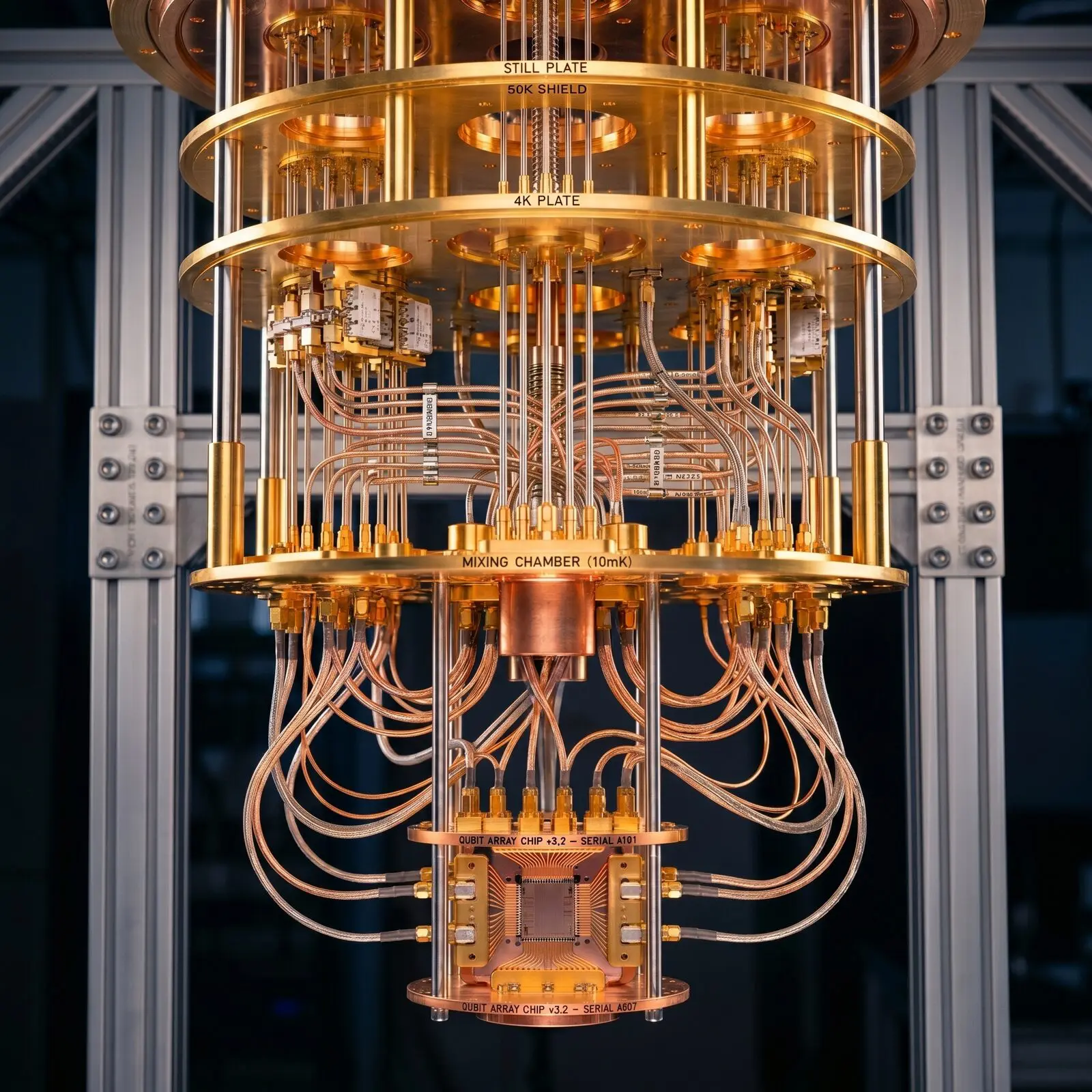
The physical mechanism behind quantum decoherence is entanglement. When a qubit in superposition interacts with environmental degrees of freedom (air molecules, thermal radiation, substrate phonon modes), the system’s state evolves into an entangled state of the qubit + environment in which the qubit’s |0⟩ component is correlated with one environment state and the qubit’s |1⟩ component is correlated with a different environment state. Tracing out the environmental degrees of freedom (mathematically averaging over all possible environment configurations) leaves the qubit in a reduced density matrix with suppressed off-diagonal coherence elements. The reason the trace-out is effectively irreversible is information access. The environmental degrees of freedom are far too numerous and too inaccessible to track in practice; tracking the state of every air molecule in a laboratory or every thermal photon in a dilution refrigerator is computationally impossible. From the experimenter’s perspective the lost coherence information has effectively become inaccessible, and the qubit transitions from a pure superposition to a classical statistical mixture. This is the canonical structural explanation for why macroscopic objects do not appear to be in superposition: the environmental coupling is so strong and the decoherence timescale so short that the trace-out happens essentially instantaneously.The three coherence-time benchmarks
The field uses three standard benchmarks to describe how long a qubit stays coherent, and the order they decay in is fixed: T1 sets the absolute ceiling, T2 the practical computing window, and T2* the raw free-running lifetime. A qubit cannot maintain phase information longer than it maintains energy, so the chain T1 ≥ T2 ≥ T2* holds for every modality.
T1 is the energy relaxation time, the timescale over which an excited qubit |1⟩ decays back to |0⟩ through spontaneous emission or coupling to a thermal bath, and it is sometimes called the longitudinal relaxation time. T2 is the dephasing time measured in a Hahn-echo experiment, which refocuses slow noise and so reports the qubit’s transverse coherence under realistic gate sequences. T2* is the Ramsey or free-induction decay time, shorter than T2 because it folds in inhomogeneous broadening and slow drifts that an echo would have cancelled out.
The three numbers are tied together by the canonical relation 1/T2 = 1/(2 T1) + 1/Tφ, where Tφ is the pure dephasing time from environmental noise that is not energy relaxation. In practice T2 is the figure to watch for circuit depth, T2* is the figure that single-qubit Ramsey calibrations chase, and T1 quietly caps both from above.
T1, T2, and T-phi: the three timescales
Quantum decoherence is characterised by three primary timescales that every commercial quantum-hardware vendor reports. T1 is the energy-relaxation time: the timescale over which an excited qubit in state |1⟩ decays to the ground state |0⟩, transferring its excitation energy to the environment. T2 is the dephasing time: the timescale over which the relative phase between the α|0⟩ and β|1⟩ amplitudes of a qubit superposition randomises through environmental coupling. Tφ (T-phi) is the pure-dephasing time: the part of T2 that does not come from energy relaxation, the dephasing process unrelated to T1.Why coherence time matters operationally
The operational consequence is the maximum circuit depth a qubit can support before decoherence destroys the computation. A quantum algorithm that needs to apply N gates, each taking time , requires the qubit to stay coherent for at least N * . With superconducting gate times of 50 nanoseconds and T2 of 100 microseconds, a qubit can support roughly 2,000 sequential gates before decoherence dominates. Larger algorithms need either longer T2 (impossible in many cases) or quantum error correction (the industry standard answer).The mathematics: density matrices and the Lindblad equation
The mathematical machinery for quantum decoherence centres on the density matrix ρ and the Lindblad master equation. A pure quantum state is described by a state vector |ψ⟩ in Hilbert space; the corresponding density matrix is the outer product ρ = |ψ⟩⟨ψ|, a rank-1 projector. A mixed quantum state is a probability mixture of pure states, written ρ = Σ |ψ_i⟩⟨ψ_i| with non-negative weights summing to one. The off-diagonal elements of the density matrix (the coherences) encode the phase relationships between basis states, and these are what decoherence destroys.The canonical noise model in simulators
Quantum simulators model decoherence by applying quantum channels rather than perfectly unitary gates. The standard approach is to express each noise process as a set of Kraus operators that act on the density matrix between ideal gate operations, which keeps the simulation tractable on a classical computer while reproducing the dominant decoherence effects measured in hardware.
Three channels do most of the work in production simulators. The amplitude-damping channel takes T1 as its parameter and models energy relaxation back to |0⟩, the phase-damping channel takes Tφ as its parameter and models pure dephasing without energy loss, and the depolarising channel mixes the qubit toward the maximally mixed state with a single error probability p that is easy to fit to benchmarking data.
The major open-source simulators expose these channels directly. Qiskit Aer supplies amplitude_damping_error, phase_damping_error and depolarizing_error; Cirq offers AmplitudeDampingChannel, PhaseDampingChannel and DepolarizingChannel; PennyLane wraps the same set under qml.AmplitudeDamping, qml.PhaseDamping and qml.DepolarizingChannel. Production noise models combine all three with measurement error and per-gate calibration data taken straight from the live hardware.
Depolarising, amplitude-damping, and phase-damping channels
Quantum decoherence on a single qubit is captured by three canonical error channels that capture most of the experimentally-relevant physics. Each channel is a completely-positive trace-preserving (CPTP) map on the qubit density matrix, parameterised by an error probability p.| Channel | Effect | Physical origin |
|---|---|---|
| Depolarising | Replace qubit with maximally mixed state with probability p | Generic gate errors, random noise |
| Amplitude-damping | |1⟩ decays to |0⟩ with probability p | Energy relaxation (T1 process) |
| Phase-damping | Off-diagonal coherences decay with probability p | Pure dephasing (Tφ process) |
| Bit-flip | X gate applied with probability p | Symmetric depolarising approximation |
| Phase-flip | Z gate applied with probability p | Pure dephasing in Z basis |
In the operator-sum representation, the depolarising channel acts on the density matrix through four Kraus operators built from the identity and the three Pauli matrices, while amplitude-damping and phase-damping each need only two. The amplitude-damping operators encode the asymmetry of |1⟩→|0⟩ relaxation (the γ parameter is set by T1), and the phase-damping operators encode pure phase erosion (λ is set by Tφ).
Decoherence times across the seven hardware modalities
Reported T2 times in 2026 quantum hardware span six orders of magnitude across the seven major modalities. The published numbers give a clean overview of which modalities maintain superposition longest and which need the most aggressive decoherence mitigation.| Modality | Typical T1 | Typical T2 | Leading vendor |
|---|---|---|---|
| Superconducting transmon | 100-300 µs | 80-300 µs | IBM Heron, IQM Radiance |
| Trapped ion (hyperfine) | minutes-hours | seconds-minutes | IonQ Forte, Quantinuum Helios |
| Neutral atom (Rydberg) | seconds | 1-10 seconds | QuEra Aquila, Atom Computing Phoenix |
| Photonic qubit | transit-time limited | transit-time limited | PsiQuantum, Xanadu |
| Silicon spin (electron) | 1-10 ms | 0.1-1 ms | Diraq, Quantum Motion, SQC |
| Cat qubit (bosonic) | 1 hour bit-flip lifetime | seconds (phase) | Alice & Bob Boson 4 |
| NV-centre diamond | 1-10 ms (electronic) | 1-10 ms (electronic) | Quantum Brilliance |
Mitigation: dynamical decoupling, error mitigation, error correction
Three architectural strategies fight quantum decoherence in production hardware, working at very different levels of the stack. Dynamical decoupling operates on the pulses themselves, error mitigation operates on the post-processed outputs, and quantum error correction operates on the logical-qubit encoding.
Dynamical decoupling
Dynamical decoupling applies a sequence of carefully timed gates, typically X-gate pulses at intervals shorter than the noise correlation time, that average out the environmental coupling and effectively extend the qubit’s coherence time. The simplest sequence is the Carr-Purcell-Meiboom-Gill (CPMG) routine borrowed from nuclear magnetic resonance, which lifts T2 from its bare Ramsey value (T2*) to a longer echoed value (T2_CPMG) by cancelling slow environmental fluctuations.
Quantum-control vendors ship production dynamical-decoupling protocols out of the box. Q-CTRL Boulder Opal, IBM Qiskit Dynamics and Quantum Machines OPX all let users insert decoupling sequences into ordinary circuits without writing pulse-level code themselves.
Quantum error mitigation
Quantum error mitigation operates one level above the hardware and extracts cleaner expectation values from noisy circuits without encoding the qubits in a logical-qubit code. Q-CTRL Fire Opal, Qedma QESEM and Algorithmiq error-mitigation software ship on commercial NISQ-era hardware and report up to 10,000x performance improvements on specific workloads.
The approach is hardware-agnostic post-processing rather than physical error suppression. It has become the canonical near-term answer for running useful quantum-chemistry, finance and optimisation workloads on today’s noisy hardware while the field waits for full error correction.
Quantum error correction
Quantum error correction is the long-run answer to decoherence. A QEC code encodes a logical qubit into many physical qubits in a way that lets the system detect and correct decoherence-induced errors faster than they accumulate, and the threshold theorem proves that any code with physical-qubit error rate below the code-specific threshold can be scaled to suppress logical-error rates arbitrarily.
The 2025 to 2026 logical-qubit demonstrations prove the approach works in practice. Google Willow, QuEra 96 LQ, Quantinuum Helios 48 LQ and Atom Computing 24 LQ have each shown logical qubits beating their physical-qubit error rates. See our what is quantum error correction and top quantum hardware companies guides for the full picture.
Decoherence and the measurement problem
The measurement problem in foundations of quantum mechanics asks why quantum measurements seem to produce definite classical outcomes despite the underlying unitary evolution being deterministic and reversible. The decoherence framework provides a partial answer: a quantum system interacting with a measurement apparatus and the broader environment quickly becomes effectively classical because the off-diagonal coherence elements of the joint density matrix decay on a timescale much shorter than any human-scale measurement could resolve. The remaining open question is the preferred-basis problem (why measurements project onto specific basis states rather than arbitrary superpositions) and the outcome problem (why a single outcome is observed rather than the full superposition of outcomes). The Wojciech Zurek einselection programme addresses the preferred-basis problem by showing that the environment naturally selects a pointer basis through the structure of the system-environment interaction. The outcome problem remains genuinely controversial across competing interpretations of quantum mechanics, including the Copenhagen interpretation, many-worlds, consistent histories, and the broader interpretations covered in our many-worlds interpretation guide.Pointer states are the practical takeaway. The environment continuously monitors observables that commute with the system-environment interaction Hamiltonian, and those observables (position for a dust grain, energy for an atom in a cavity) become the basis in which the world looks classical. Decoherence does not solve the measurement problem, but it explains why the question only feels acute for isolated quantum systems and never for everyday objects, whose coherence times are smaller than 10-20 seconds.
Frequently asked questions
What is quantum decoherence in simple terms?
Quantum decoherence is the process by which a qubit in superposition loses its coherent quantum information through interaction with its environment, transitioning from a clean quantum state to an effectively classical statistical mixture. The mechanism is entanglement: the qubit’s superposition becomes entangled with environmental degrees of freedom (air molecules, thermal radiation, magnetic fluctuations), and tracing out the environment leaves the qubit in a classical mixture. The information is not destroyed in any fundamental sense; it just leaks into the environment in a form that is practically impossible to recover. Decoherence is the canonical reason macroscopic objects do not appear to be in superposition and the canonical reason every commercial qubit needs error correction.What is the difference between T1 and T2?
T1 is the energy-relaxation time: the timescale over which an excited qubit in state |1⟩ decays to the ground state |0⟩ by transferring its excitation energy to the environment. T2 is the dephasing time: the timescale over which the relative phase between the α|0⟩ and β|1⟩ amplitudes of a qubit superposition randomises. The constraint T2 less-than-or-equal-to 2 * T1 always holds because a pure superposition can only stay coherent as long as the underlying populations are stable. Most physical qubits run at T2 substantially below 2 * T1 because pure dephasing (Tφ) typically dominates over energy relaxation, and the canonical relationship is 1/T2 = 1/(2 * T1) + 1/Tφ.How long does quantum coherence last in 2026 hardware?
Reported T2 times in 2026 quantum hardware span six orders of magnitude across the seven major modalities. Trapped ion (IonQ Forte, Quantinuum Helios) holds the deepest coherence-time lead at seconds to minutes in hyperfine ground states. Neutral atom (QuEra, Pasqal, Atom Computing) reaches tens of seconds. Silicon spin (Diraq, Quantum Motion, SQC) and NV-centre diamond (Quantum Brilliance) run at milliseconds. Superconducting transmons (IBM Heron, IQM Radiance, Google Willow, Rigetti) cluster at hundreds of microseconds. Photonic qubits do not have a well-defined T1/T2 because the decoherence happens through photon loss and mode-mismatch rather than population relaxation. Cat qubits (Alice & Bob Boson 4) report a bit-flip lifetime of one hour with a much shorter phase-flip lifetime.How do quantum computers fight decoherence?
Three architectural strategies fight quantum decoherence in production hardware. Dynamical decoupling applies a sequence of carefully-timed control pulses that average out the environmental coupling and extend the qubit’s effective coherence time; the simplest variant is the Carr-Purcell-Meiboom-Gill (CPMG) sequence. Quantum error mitigation operates above the hardware and extracts cleaner expectation values from noisy circuits without encoding qubits in a logical-qubit code; Q-CTRL Fire Opal, Qedma QESEM, and Algorithmiq ship production error-mitigation software with up to 10,000x performance improvements. Quantum error correction is the long-run answer: a QEC code encodes a logical qubit into many physical qubits and corrects decoherence-induced errors faster than they accumulate, scaling to fault-tolerant quantum computing through the threshold theorem.What is the Lindblad master equation?
The Lindblad master equation is the canonical mathematical tool for describing the time evolution of an open quantum system’s density matrix as a sum of unitary evolution plus dissipative terms. The standard form is dρ/dt = -i[H, ρ] / hbar + Σ_k ( ρ -dagger – (1/2){-dagger , ρ}), where H is the system Hamiltonian and the are Lindblad jump operators that capture the dissipative interaction with the environment. The Lindblad form is the most general Markovian (memoryless) quantum master equation that preserves trace and complete positivity of the density matrix, and every commercial quantum-circuit simulator (Qiskit Aer, Cirq, PennyLane, Q-CTRL Boulder Opal) includes Lindblad simulators for hardware-noise modelling.What is a density matrix?
A density matrix ρ is the mathematical object that represents the state of a quantum system, generalising the state vector |ψ⟩ to handle both pure quantum states and statistical mixtures. A pure state is represented by ρ = |ψ⟩⟨ψ|, a rank-1 projector with off-diagonal coherences. A mixed state is a probability-weighted sum of pure states, ρ = Σ |ψ_i⟩⟨ψ_i|, where the off-diagonal coherences are partially suppressed depending on the degree of mixing. Decoherence is the process that suppresses the off-diagonal elements of the density matrix toward zero, taking a pure-state density matrix to an effectively classical statistical-mixture density matrix. The density matrix formalism is essential for any rigorous treatment of quantum noise and decoherence.Why does Schrödinger’s cat not stay in superposition?
Schrödinger’s 1935 thought experiment imagined a cat in an entangled superposition of alive and dead, scaled up from a single radioactive-atom quantum system. The modern resolution is decoherence. A cat is a macroscopic object with roughly (10)^25 particles interacting strongly with the air, the box, the radioactive material, the Geiger counter, and the broader thermal environment, and these interactions destroy the superposition essentially instantaneously. The cat’s reduced density matrix transitions from a pure superposition to a classical statistical mixture on a timescale far shorter than any human-scale measurement could resolve. The cat is therefore not in superposition in any practical experimental sense because the environment has already effectively measured the cat’s state through countless interactions.What is the amplitude-damping channel?
The amplitude-damping channel is one of the three canonical single-qubit error channels in quantum information theory, capturing the energy-relaxation (T1) process by which an excited qubit in state |1⟩ decays to the ground state |0⟩. The mathematical form is a CPTP map with two Kraus operators that interpolate between perfect identity (no decay) and complete decay to |0⟩ with probability p. The amplitude-damping channel is the natural model for spontaneous emission in atomic and trapped-ion qubits, for photon loss in photonic qubits, and for the energy-relaxation T1 process in superconducting transmons. The complementary phase-damping channel models pure dephasing (Tφ) without energy loss, and the combined dynamics on real hardware is typically a weighted sum of amplitude damping plus phase damping.Who discovered quantum decoherence?
The decoherence concept arrived in physics through three parallel developments. H. Dieter Zeh introduced the framework in his 1970 paper “On the Interpretation of Measurement in Quantum Theory” published in Foundations of Physics, recognising that macroscopic objects interact too strongly with their environments to maintain quantum superposition. Wojciech Zurek formalised the einselection programme through the 1980s and 1990s, showing that environmental interactions naturally select a preferred classical basis through a process he termed einselection. Serge Haroche at ENS Paris experimentally observed mesoscopic-superposition decoherence in microwave-cavity-QED experiments in the 1990s, sharing the 2012 Nobel Prize in Physics with David Wineland. Maximilian Schlosshauer’s 2004 Reviews of Modern Physics survey consolidated the modern theoretical landscape.How does decoherence relate to quantum error correction?
Quantum error correction is the engineering response to quantum decoherence. A QEC code encodes a logical qubit into many physical qubits in a way that lets the system detect and correct decoherence-induced errors (bit flips from amplitude damping, phase flips from pure dephasing, depolarising errors from generic noise) faster than they accumulate. The threshold theorem says that any QEC code with physical-qubit error rate below the code-specific threshold can be scaled to suppress logical-error rates arbitrarily, the foundation of fault-tolerant quantum computing. The 2025-2026 logical-qubit demonstrations from Google Willow (superconducting surface code), QuEra (96 logical qubits on neutral-atom qLDPC), Quantinuum Helios (48 LQ trapped-ion), and Atom Computing (24 LQ Microsoft Azure) prove the approach beats decoherence in practice.What is dynamical decoupling?
Dynamical decoupling is a quantum-control technique that fights decoherence by applying a sequence of carefully-timed control pulses (typically X gates) at intervals shorter than the environmental noise correlation time. The pulses effectively average out the environmental coupling and extend the qubit’s effective coherence time from T2* (the bare dephasing time) to (the dynamically-decoupled value), often by an order of magnitude or more on real hardware. The simplest sequence is the Carr-Purcell-Meiboom-Gill (CPMG) sequence from nuclear magnetic resonance; more advanced sequences include Uhrig dynamical decoupling and concatenated sequences that target specific noise spectra. Quantum-control vendors (Q-CTRL Boulder Opal, IBM Qiskit Dynamics, Quantum Machines OPX) ship production dynamical-decoupling protocols on commercial hardware.Does decoherence destroy quantum information forever?
Decoherence does not destroy quantum information in any fundamental sense; the information leaks from the qubit into the environment and is in principle still accessible if you could track every environmental degree of freedom the qubit ever interacted with. In practice the environmental degrees of freedom are far too numerous and inaccessible to track, so from the qubit’s perspective the information is irrecoverably lost on practical experimental timescales. The structural answer is that decoherence is reversible in principle but irreversible in practice. Quantum error correction works by intercepting the decoherence-induced errors before the information leaks to inaccessible environmental degrees of freedom, encoding the logical information in a redundant physical-qubit code that resists local decoherence.


See today’s quantum computing news on Quantum Zeitgeist for the latest breakthroughs in qubits, hardware, algorithms, and industry deals.