This post discusses the potential of using Quantum Variational Circuits as feature extractors and as additionally as classification layers in a classical neural network. There is implementation in qiskit with code such that the user can also run working code.

It’s assumed that the reader will have a basic understanding of machine learning. Regarding requisite quantum knowledge, it will be great if the user has a reasonable background in quantum physics. Otherwise, the reader can click on the links to learn about concepts and fundamentals.

Aims

• Review basics of linear classification.
• Learn how to transform a basic classical classification problem into a quantum one.
• Learn how to use quantum trainable circuits within a classical neural network.

Classical machine learning and computer vision

Image Classification is one of the main tasks in Computer Vision. The sole purpose of this task is to assign a unique label or category to each image. Before the huge advancements in Deep Learning and GPUs, Image Classification relied on image processing techniques such as Histogram of Oriented Gradients [1], Speeded-Up Robust Features [2] to extract distinctive features from each image and then use one of the Machine Learning algorithms such as Support Vector Machines, Random Forests, K-Nearest Neighbor, or Extra-Trees.

Basics of supervised learning

In any supervised machine learning pipeline, you shall have a matrix where is the number of samples or images in this case and is the number of features that you have extracted earlier. In some cases would be the number of the dimensions of the flattened image i.e if your image is then will be .
This means that you will use the whole image as an input sample to your learning algorithm. This usually happens when you use any deep learning algorithm such as the Multi-Layer perceptron depicted in figure 1 or Convolutional Neural Networks as in figure 2.

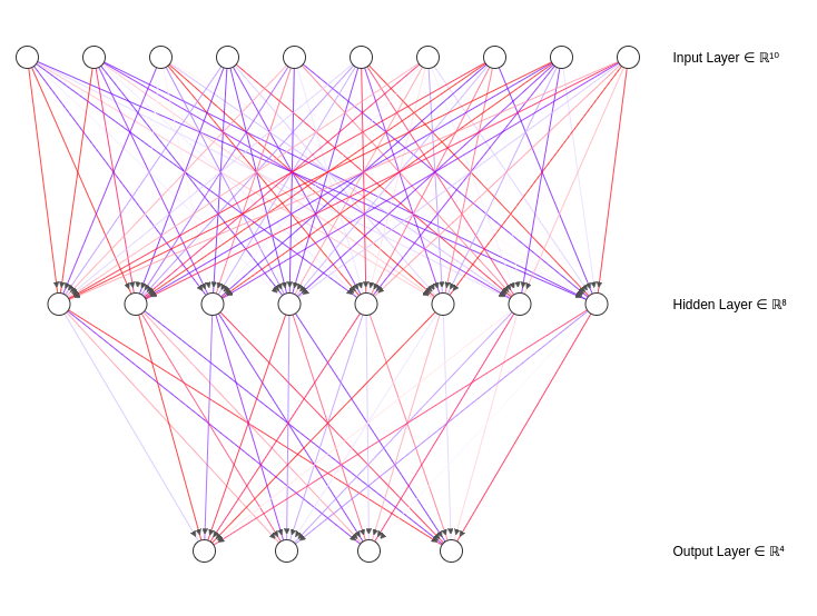
Besides the matrix that contains your data, you will also have a label vector where is the number of categories that you want to classify. The role of the machine learning algorithm is to perform some operations to map the input data to the correct label. Simply enough

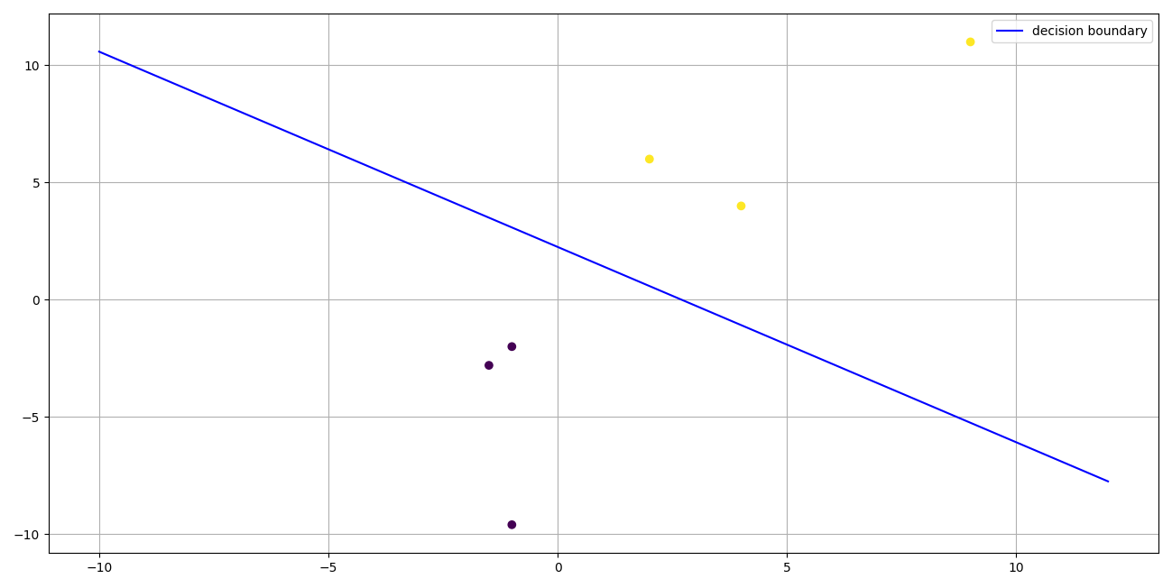
That function can be a simple straight line like this equation: where , and are the slope or the weights and the bias “the ” that should be updated during the backpropagation. By forcing a condition on the output from this function i.e. if the total output of is bigger than then the label will be otherwise it will be . So, the final decision function would be . We can easily use this function to classify two labels where the separation is pretty easy. Figure 3 depicts the concept of a straight line classifying two categories.

For more information about linear models and when to say if a model is linear and linear in what exactly, I do recommend this CalTech course by Prof. Yaser Abu-Mostafa. You can find the videos, lecture slides and Q&A sessions.

The Universality of Neural Networks

Going back to figure 2, each node actually performs the function plus an activation function such as the or . According to the Universality Theorem [3,4], we can approximate any continuous function if there are enough nodes and at least one hidden layer. Besides, the in each node is updated iteratively, this means the network can capture hidden patterns in the data and can be used as feature extractors. As a result, we can no longer say that neural networks are linear classifiers. This also means that complex – aka non-linear separable – datasets can be efficiently classified by neural networks. On the other hand, one needs a transformation such as a polynomial function or a radial basis function to map the features into a higher and richer Hilbert Space. A wonderful explanation for this is the kernel trick in SVMs, or if you are already familiar with these concepts you may find the following Colab notebook – where I used a single Qubit to classify a complex binary dataset using Qiskit – entertaining.

Quantum machine learning

Speaking of which, qubits are the new hype of the computing world as they propose a much higher capacity of information processing and also a faster run times. If you want to know more about how to represent your information using qubits, Qiskit-textbook is the right place to start. Other than that, these two slides are very good if your mathematics background is a bit good pdf_1, pdf_2. They provide you with the basics of qubit representation and also how to manipulate the qubit.

The problem with the current quantum technology is that quantum computers are not very mature and they are prone to noise. This limits their capabilities severely. On the other hand, Quantum Variational Circuits [5,6] avoid most of the classical operations such as addition, and information memorizing. Moreover, the quantum gradients [7] of such circuits can be calculated efficiently.

Figure 4 shows the basic follow of how to make the quantum circuit trainable to act as a neural network. The following steps explain the training process:

1. Encode the classical data into the quantum circuit “Quantum Embedding“.
2. Apply the variational quantum circuit to your data.
3. Measure the desired qubits to form your output.
4. Calculate the cost function of your algorithm.
5. Update the weights of the quantum circuit.
6. Repeat until convergence.

Let’s break these 6 steps one by one. In 2018 a paper called “Circuit-Centric Quantum Classifiers” [8] appeared on Arxiv. The authors presented a way to mimic the behaviour of classical neural networks. As shown in figure 5, you encode the classical data into the quantum circuit. Then you apply a linear unitary operation. After that, a non-linear operation is applied which is the measurement “we will get to that later”. Finally, we process the output of the quantum circuit to establish the same rule of the binary classification of the straight line, i.e. the function .

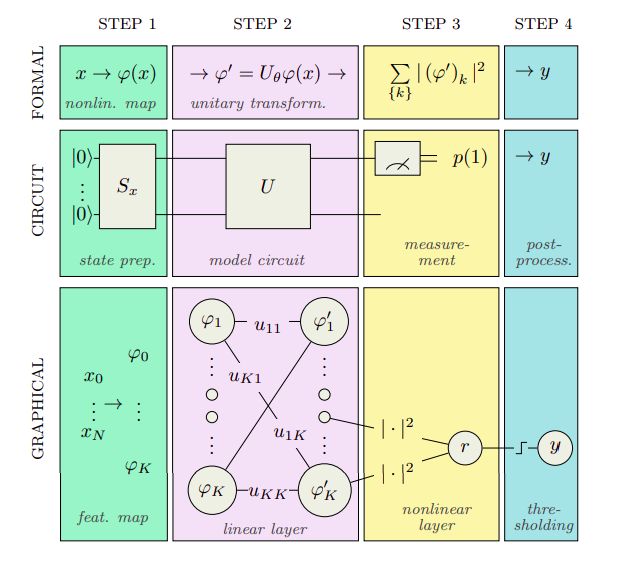
First, encoding any classical data into a complex Hilbert space – in which the wave function of the quantum circuit lives – equals the performing of a feature map to transform the complex data into a much more richer feature space, i.e. the Kernel Trick is implied [8,9]. The authors in the paper use a technique called Amplitude Encoding. Amplitude encoding provides an incredible feat because if the number of the features is then the required number of qubits is . This is due to the fact that we encode the features into the amplitudes of the available quantum states as follows:

, where and obey the following relation: .

This can be summed by the following expression: .

Hence, the above encoding requires us to normalise the input features by the norm. The norm of a sample is calculated by:

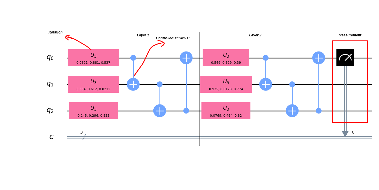
Second, the utilised unitary operation is a linear operation and it mimics the multiplication . The authors used a parameterised gate with 3 variables “the gate or the Rotation gate”. this gate can be decomposed into: . Physically, this means rotating the state vector of a single qubit around the X, Y and Z axes. The following website contains some visualisations that can give you a hint to what is happening. They also used a 2 qubit gate which is called a CNOT gate. This gate enables us to make the qubits interact with each other resulting in an entanglement. As a matter of fact, Controlled gates can be decomposed by any unitary gate, i.e. we can apply Controlled-Z, Controlled-Y, and even Controlled-Rotation.

Third, Measuring or trying to extract any kind of information is a non-linear process; because it can not be inverted and it does destroy the superposition of the quantum state. But it gives some insights about the quantum state itself. The authors used a simple measurement procedure where they want to compute if the first qubit is in the state, this can be achieved by measuring the Z observable “Pauli Z Operator” for the first qubit as follows where is a unitary matrix:

.

The outcome from the observable is a continuous bounded output between this interval . You may find this PDF a bit useful to understand more about measurements. After the measurement, you can classically process it by adding a bias term or applying any function you want as explained in the paper in equation 1. The remaining steps are the same as we would do for a classical neural network.

Figure 6 shows the main architecture of the quantum circuit. By increasing the number of layers we can increase the flexibility of the circuit to model any function. We can also modify the connections between the controlled operations so that can be connected with , i.e. this is another hyperparameter that can contribute to the output. This circuit can also encode up to 8 features per sample using the amplitude encoding scheme, which represents a polynomial of the 1st degree. Please check [9] for more details. The paper discusses other hyperparameters such as dropout.

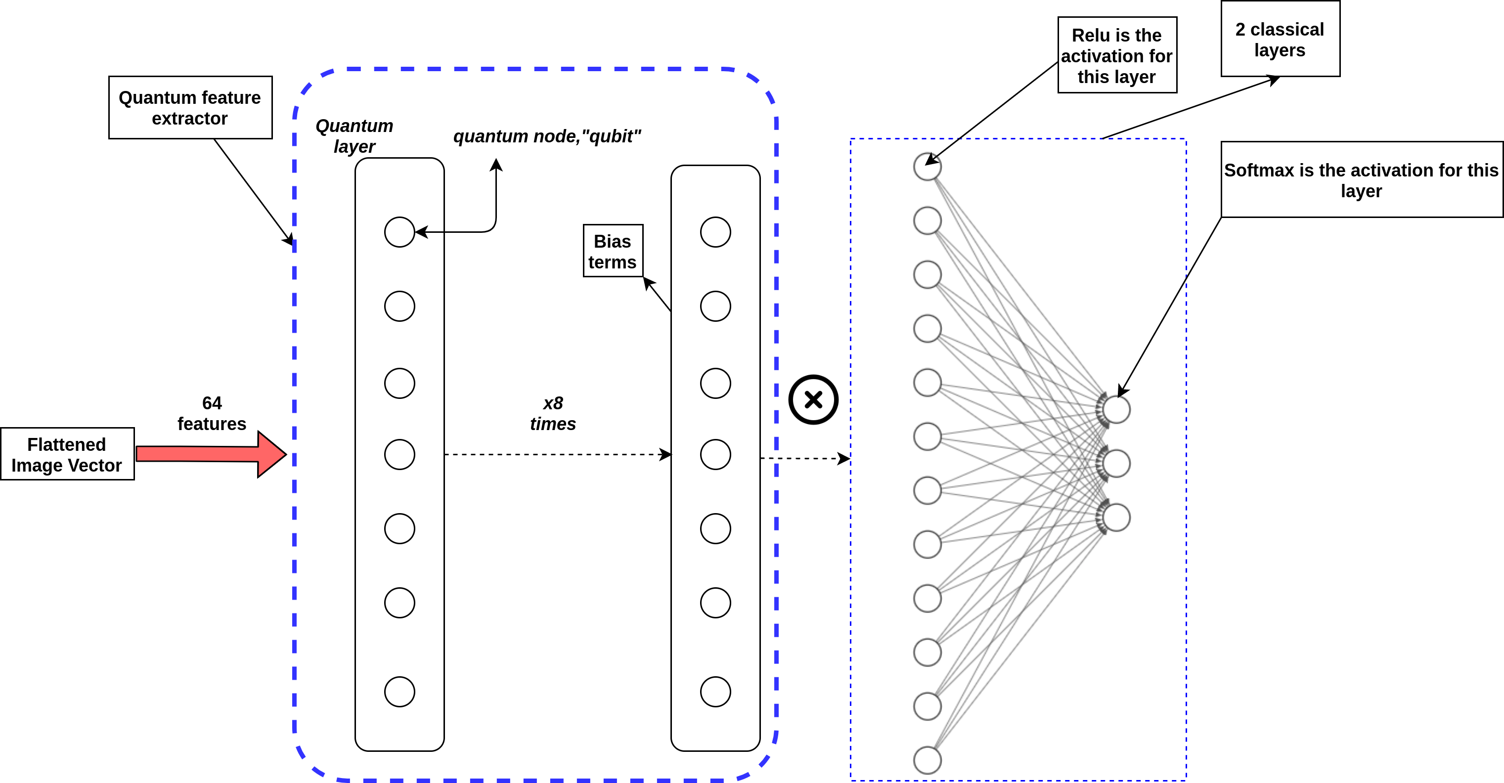
This quantum classifier is perfect for binary classification and can be used in a One Vs All fashion for multiclass classification problems as described in the following links {1,2,3}. Or, we can measure multiple qubits and form an output vector and apply a softmax function and then compute the loss by a cross-entropy function. The only problem with the softmax approach is that the probabilities from the quantum circuit follow a random uniform distribution and it’s bounded by a relatively small interval. This may cause a saturation and high loss value from the cross-entropy function. To overcome this we may multiply the output by a factor to scale it or we may add a classical layer with its weights and bias to be optimised later on by an iterative method like the gradient descent alongside with the quantum parameters.

Finally, we’ve reached the main purpose of the tutorial. Instead of using the quantum circuit as a simple classifier, we will follow it by 2 classical layers so that the quantum circuit would act as a trainable feed-forward neural network. Figure 7 shows the full architecture of the classifier. This means that we will measure 7 qubits and then add the bias terms. After that, we will connect each of the 7 outcomes with the following layer to perform the dot products and the activation function just as we do in classical neural networks.

The advantages of this classifier are the following:

1. It’s highly compact, i.e. with a very small number of qubits we managed to encode 64 features. In a typical neural network, we would initialize the input layer with 64 units.
2. With a small number of parameters, we managed to achieve a very high F-1 score “1”. Typical neural networks require huge numbers of units to achieve the same.
3. Data encoding can introduce an incredible feat for convergence speed.
4. In [10], the authors used a similar approach to mimic the convolution neural networks mechanism. So, instead of flattening the image, a quantum circuit convolves the images like a filter to extract the quantum features and then a classical layer and so on.

The disadvantages:

1. According to [11] encoding the data may require lots of rotation gates and controlled operations.
2. Using lots of Controlled operations is not favourable; since the current quantum computers are not immune against noise and some of them have high error readouts for 2-qubit gates.

Software Implementation

The problem we are trying to solve is classifying the first 3 digits of the MNIST dataset. Actually, we will use a small modified version of it for simplicity. Here is an example of how to classify it with SVM using Scikit-Learn library.

Regarding the quantum part of the classifier, we will use Pennylane [12]. Pennylane is a quantum machine learning library that is compatible with many quantum frameworks and also hardware agnostic. It’s also integrated with Autograd so that we will not pay attention to calculating the gradients. It already computes the gradients for both the quantum and classical parts.
Pennylane also provides some amazing templates such as the amplitude encoding template and Strongly Entangling layers template. The following code shows you how to implement the circuit in figure 6:

import pennylane as qml
dev = qml.device("default.qubit", wires=3)
weights = qml.init.strong_ent_layers_uniform(n_layers=2, n_wires=3,low=0,high=1,seed=0)

@qml.qnode(dev)
def qclassifier(weights, X=None):
    qml.templates.AmplitudeEmbedding(X,wires=list(range(3)), pad=0.0,normalize=True)
    qml.templates.StronglyEntanglingLayers(weights, wires=list(range(3)))
    return [qml.expval(qml.PauliZ(i)) for i in range(1)]

The line where we defined the backend device is very important since we can use real backends from IBM quantum computers, or Rigetti’s. But, in our tutorial we used a simulator called Qulacs. It’s a high-speed backend simulator which uses GPUs. Pennylane already provides many plugins alongside Qulacs. I urge you to explore them and try different settings.
Lastly, in this Colab notebook, you will find the implementation and how to train the classifier yourself. There is no need for any setups everything has been taken care of for you. And this is the main repo.

If you want to code the same architecture with Qiskit then you might want to extract the expectation values from the subsystems of the quantum circuit. Qiskit aqua modules have these functions already implemented for you.

Summary

We’ve covered the basic implementation of [8] and how this quantum classifier can be used in multi-class classification. We’ve also mentioned that this classifier acts as a feed-forward neural network with increasing the number of its layers.
Then we’ve combined this classifier with a classical neural network to act as a feature extractor before the main classification layer. This actually opens up many different possibilities to use the rich quantum Hilbert space in machine learning in general.

The notebook is made by Alexandria Quantum Computing Group. This is an academic group based in Alexandria University, Egypt. The group is focused on quantum technologies and primarily quantum search algorithms. The author of the post is Kareem El-Safty. I’m an Artificial Intelligence Engineer and I’m doing my research in the intersection between physics and machine learning. Please feel free to contact me or post a comment below.

Till the next time.

References

1. Histograms of oriented gradients for human detection. DOI: 10.1109/CVPR.2005.177. online version
2. Speeded-Up Robust Features (SURF). DOI: 10.1016/j.cviu.2007.09.014. online version
3. Approximation by Superpositions of a Sigmoidal Function. DOI: 10.1007/BF02551274. online version
4. Multilayer feedforward networks are universal approximators. DOI: 10.1016/0893-6080(89)90020-8. online version
5. A variational eigenvalue solver on a quantum processor. DOI: 10.1038/ncomms5213. online version
6. The theory of variational hybrid quantum-classical algorithms. DOI:
   10.1088/1367-2630/18/2/023023. online version
7. Evaluating analytic gradients on quantum hardware. DOI: 10.1103/PhysRevA.99.032331. online version
8. Circuit-centric quantum classifiers.  arXiv:1804.00633v1
9. Supervised Learning with Quantum Computers. DOI: 10.1007/978-3-319-96424-9.
10. Quanvolutional Neural Networks: Powering Image Recognition with Quantum Circuits. arXiv:1904.04767
11. Transformation of quantum states using uniformly controlled rotations. arXiv:quant-ph/0407010
12. PennyLane: Automatic differentiation of hybrid quantum-classical computations. arXiv:1811.04968